Search for articles:
Saad B. Aziz , Ayman M. Okeil
Corresponding authors:
Received: 2017-06-24
Online: 2018-01-10
Copyright: 2018 Editorial board of Acta Metallurgica Sinica(English Letters) Copyright reserved, Editorial board of Acta Metallurgica Sinica(English Letters)
More
Abstract
This paper presents a new thermomechanical model of friction stir welding which is capable of simulating the three major steps of friction stir welding (FSW) process, i.e., plunge, dwell, and travel stages. A rate-dependent Johnson-Cook constitutive model is chosen to capture elasto-plastic work deformations during FSW. Two different weld schedules (i.e., plunge rate, rotational speed, and weld speed) are validated by comparing simulated temperature profiles with experimental results. Based on this model, the influences of various welding parameters on temperatures and energy generation during the welding process are investigated. Numerical results show that maximum temperature in FSW process increases with the decrease in plunge rate, and the frictional energy increases almost linearly with respect to time for different rotational speeds. Furthermore, low rotational speeds cause inadequate temperature distribution due to low frictional and plastic dissipation energy which eventually results in weld defects. When both the weld speed and rotational speed are increased, the contribution of plastic dissipation energy increases significantly and improved weld quality can be expected.
Keywords:
Friction stir welding (FSW) has generated widespread attention after its invention by The Welding Institute in 1991 [1]. In FSW, there is absence of melting or fusion during the welding process itself; thus, this welding is free of high heat input, and eventual melting, and solidification defects. Moreover, due to the absence of filler material and the absence of fumes that are generally produced in the traditional fusion arc welding, the FSW process is considered to be environmentally green. Furthermore, FSW joints generally have higher mechanical properties and lower post-weld tensile residual stress than conventional fusion welding. The FSW process starts by plunging a rotating pintool with a shoulder into the workpiece at the joint between two metal pieces to be joined as shown in Fig. 1. The rotational motion of the pintool causes frictional heat and consequently large plastic deformations due to material stirring in the workpiece. The shoulder also helps prevent the material from being expelled out of the weld center. A backing plate placed at the bottom of the workpiece prevents its movement and deformation while welding.
Fig. 1 Schematic representation of friction stir welding (FSW) process [
Previous work on modeling FSW process can be divided into two main categories: pure thermal models and coupled thermomechanical models, which account for the interaction between thermal and mechanical deformation. The pure thermal models only compute temperature fields. On the other hand, thermal and deformation coupled models may be classified into two types, namely computational solid mechanic (CSM)-based models and computational fluid dynamic (CFD)-based models [3]. A Lagrangian formulation is commonly used in CSM models, and an Eulerian formulation is commonly used in CFD models. Lagrangian formulation permits mesh and material to move at the same time, which enables tracking surfaces. Its limitations lay in the difficulty to achieve convergence when elements become severely distorted. On the other hand, in the Eulerian approach materials move through the mesh. The shortcoming of this approach is that it is challenging to tracking surface and the boundary conditions. Nevertheless, distortion of mesh is not a problem since mesh distortion never occurs in the Eulerian approach. Another approach is known as arbitrary Lagrangian-Eulerian (ALE) method which incorporates the benefit of both Lagrangian and Eulerian approach and, hence, is suitable for large deformation problem. In the arbitrary Lagrangian and Eulerian (ALE) method, the node points can be moved arbitrarily which enables the material to move independent of mesh.
Several research articles have been published so far on the aspects of thermal modeling of friction stir welding [4, 5, 6, 7, 8, 9, 10, 11, 12]. Zhang et al. [13] developed an analytical thermal model which considered all necessary steps in FSW. In the model, an inverse solution method (ISM) has been used in the analysis to calculate rate of heat generation. The extension of the proposed model by Zhang et al. [14] has been analyzed with the consequence of different weld parameters on temperature and heat generation.
An ALE formulation was employed by Zhang et al. [15] to develop rate-independent material model. However, the results did not include any discussion on plastic and frictional energy dissipation. Another rate-independent model was developed by Zhang et al. [16, 17, 18] to analyze influences of plunge force, welding speed, and rotational speed upon material flow. During FSW, influence of stick (pintool and material have the same velocity) as well as slip (pintool and material have different velocities) has been modeled assuming a slip rate of 0.5% \(({\text{Slip}}\,{\text{rate}}\left( {\text{dimensionless}} \right) = \frac{{{\text{Angular}}\,{\text{rotation}}\,{\text{speed}}\,{\text{of}}\,{\text{the}}\,{\text{contact}}\,{\text{matrix}}\,{\text{layer}}}}{{{\text{Angular}}\,{\text{rotation}}\,{\text{speed}}\,{\text{of}}\,{\text{the}}\,{\text{tool }}}})\) [19]. Buffa et al. [20] developed a continuum model using a Lagrangian-based code, DEFORM-3D™. However, it was assumed that the material properties of the workpiece (thermal conductivity and thermal capacitance) were constants, and in real life, it varies with temperature. Besides, the workpiece plate was modeled as “single block,” rather than two parts next to each other, to avoid contact instabilities. Aziz et al. [21] developed a FSW model using a rate-independent material model. The model used three different weld schedules to verify temperature profile of simulation with experimental results. Furthermore, the verified model was used to analyze the effects of different weld parameters on heat generation and its sources (friction vs. plastic deformation). Another FSW model was developed using ABAQUS by Aval et al. [22], who showed that the temperature in FSW process was distributed unevenly along the weld line.
Lasley et al. [23] developed a model to model the plunge stage of FSW only using commercial software called “Forge3.” Heurtier et al. [24] developed a semi-analytical model considering microstructure change during welding in lightweight aluminum alloy. The kinematic model was divided into two parts. One location is just below the shoulder of the tool and corresponds to the “flow arm zone.” The other zone is “nugget zone”—located in the depth zone. Grujicic et al. [25] developed a 3D flow model using a modified Johnson-Cook model which takes into consideration of the dynamic recrystallization effect during FSW. Assidi et al. [26] developed a 3D FSW model using commercial software Forge3® FE software. Two different models formulated with Eulerian and ALE techniques have been developed and compared. From the model, several conclusions were drawn. First, the arbitrary Lagrangian-Eulerian technique is in good agreement with the measured forces and tool temperature. Second, Coulomb’s friction model provides better result than Norton friction model. Hamilton et al. [27] developed a thermomechanical model using the Johnson-Cook material model. In order to capture material flow and high deformation underneath the pintool, authors used adaptive re-meshing technique. However, like Assidi et al. [26], the friction coefficient between the pintool and workpiece was considered to be constant in this study. In reality, the friction coefficient is temperature dependent; as the temperature increases, the friction coefficient decreases [28].
Most of the thermal modeling calculates source of heat using heat flux per unit area which is distributed over the tool surface. This heat flux is inputted by the user in the model as a constant intensity or it is varied as a function of the distance from the tool’s axis. However, this type of modeling is far from real-life welding scenario and is incapable of capturing real-life friction interface between tool and the workpiece because the effect of stick/slip during FSW cannot be captured. Furthermore, strain rate dependency cannot be captured with thermal modeling. The FSW process consists of several complex physical processes. An ideal and fully thermomechanical model of FSW (1) should be temperature dependent, (2) should be able to capture tool material interface condition (stick/slip condition), and (3) needs to be strain rate dependent. Moreover, in all of the aforementioned models, only the models developed by Buffa et al. [20] and Hamilton et al. [27] simulated all three stages of FSW; however, these two models assume a temperature-independent friction coefficient.
The main objective of this current work is twofold: Foremost, to build a rate-dependent thermomechanical model which can evaluate heat generation during FSW by considering the frictional heat and plastic deformation. A major difference between the presented model and previous models published so far is that all steps of FSW processing were successfully simulated including plunge, dwell, and travel stages. And secondly, the model used a temperature-dependent friction coefficient that considers sticking/sliding conditions. Two separate experimentally obtained weld schedules have been used to validate the numerical model.
The subsequent objective of this study is to conduct a parametric study of the critical weld parameters, namely rotational speed, weld speed, and plunge rate, for furthering understanding of FSW processing. These weld schedules were selected from an earlier experimental investigation by the Louisiana State University’s research team [29].
A finite element (FE) model is developed for simulation of FSW process of aluminum alloys. The developed model is validated using experimental results taken from the FSW process of workpieces tested by the authors [29]. An I-STIR PDS-FSW machine with a fixed pintool was used in welding the workpieces selected for model validation. The experimental setup is shown in Fig. 2. Both validation weld workpieces were made of lightweight AA2219-T87 aluminum alloy, whose chemical composition is listed in Table 1.
Fig. 2 Dominant FSW process parameters and experimental setup
Table 1 Chemical compositions (wt%) of AA2219
| Element | Ti | Zn | Fe | V | Cu | Mn | Zr | Si | Mg |
|---|---|---|---|---|---|---|---|---|---|
| wt% | 0.10 | 0.10 | 0.30 | 0.15 | 6.8 | 0.40 | 0.25 | 0.20 | 0.02 |
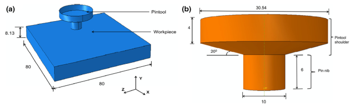
The developed finite element (FE) model consists of two simulated parts: workpiece and pintool, as shown in Fig. 3. In the model, the pintool is considered as a 3D rigid body rather than a deformable material as they are manufactured from a hardened material that can stir the workpiece metal and to avoid computational complexities. The pintool shoulder has a diameter of 30 mm and a height of 4 mm. The diameter of the pin nib is 10 mm (the part that plunges into the workpiece) and its height is 6 mm. The pintool has a tapered angle of 20°.
Fig. 3 a Finite element model of the workpiece and pintool; b dimensions of the pintool
In the model, the motion of the pintool is controlled by using a reference node. The reference node has translation, rotation, and thermal degrees of freedom. The pintool is assumed to be isothermal. The workpiece’s elastic as well as plastic behavior was modeled using strain rate-dependent material model, as in real life strain rate varies greatly during FSW [30]. As mentioned previously, no heat flux was used as a heat source in the present work. Conversely, friction between the pintool and the workpiece causes heat generation in the present model. As such, any errors or bias due to user’s choice of heat source input and distribution is eliminated. In the FEA model, the workpiece has a length of 80 mm, width of 80 mm, and thickness of 8.13 mm. The meshed model has 25,600 elements and 204,800 nodes as shown in Fig. 4. As will be described later in detail, the solid element C3D8RT used to build the model consists of eight nodes with trilinear displacement. The element C3D8RT has the capability of reduced integration and hourglass control.
Fig. 4 Schematic representation of boundary conditions of thermal analysis and meshes of the finite element model (all dimensions are in millimeter)
In the current study, a temperature- as well as strain rate-dependent material model with an elasto-plastic Johnson-Cook material law [31] has been used. The Johnson-Cook plasticity model is widely used for high strain rate deformation. The model can be represented by Eq. (1) [32],
$\sigma_{y} = \left( {A + B[\varepsilon^{{ - {\text{pl}}}} ]^{n} } \right)\left(1 + {\text{cln}}\frac{{\dot{\varepsilon }_{\text{pl}} }}{{\dot{\varepsilon }_{0} }}\right)\left(1 - \left( \frac{{T - T_{\text{ref}} }}{{T_{\text{melt}} - T_{\text{ref}} }}\right)^{m} \right),$(1)
where \(\sigma_{\text{y}}\) is the yield stress, \(\dot{\varepsilon }_{\text{pl}}\) is the effective plastic strain rate, \(\varepsilon^{{ - {\text{pl}}}}\)is the effective plastic strain, and \(\dot{\varepsilon }_{0}\) is the normalizing strain rate. Here, A, B, C, n, and m represent material/test constants, and \(T_{\text{ref}}\) and \(T_{\text{melt}}\) are reference and melting temperatures, respectively. A summary of the AA2219-T87 material property for the Johnson-Cook model is listed in Table 2.
Table 2 Johnson-Cook material plastic model input [
| A (MPa) | B (MPa) | n | m | Melting temperature (°C) [33] | Reference temp (°C) |
|---|---|---|---|---|---|
| 369 | 684 | 0.73 | 1.7 | 543 | 25 |
The present model used von Mises yield criterion. This yield criterion is expressed by Eqs. (2) and (3) [34],
$f\left( {\sigma ,\sigma_{y} } \right) = \sigma_{e} - \sigma_{y} = 0,$(2)
Where$\sigma_{\text{e}} = {\text{von}}\,{\text{Mises}}\,{\text{effective}}\,{\text{stress}} = \sqrt {\frac{3}{2}\left( {\sigma :\sigma - \frac{1}{3}{\text{tr}}\left( \sigma \right)^{2} } \right)},$(3)
\(\sigma_{\text{y}}\) is the yield strength, and \({\text{tr}}\) is the Tresca criterion.
The increments of plastic strain are determined by flow rule. In present model, an associative flow rule is used. This flow rule is expressed by Eq. (4) [32, 34];
$\left\{ {\dot{\varepsilon }_{\text{pl}} } \right\} = {\text{d}}\lambda \left\{ {\frac{\partial N}{\partial \sigma }} \right\},$(4)
where \(\left\{ {\dot{\varepsilon }_{\text{pl}} } \right\}\) is the plastic strain change, \({\text{d}}\lambda\) is the plastic strain increment magnitude, \(N\) is the plastic potential, and \(\partial \sigma\) is the stress change.
Figure. 4 shows the schematic sketch of the physical model. The initial temperature boundary condition can be represented by Eq. (5) [28];
$T\left( {x,y,z,t} \right) = T_{i} {,}$(5)
The transient heat transfer process during FSW can be represented by Eq. (6) [28];
$\rho c_{\text{p}} \frac{\partial T}{\partial t} = \frac{\partial }{\partial x}\left[ {k_{x} \frac{\partial T}{\partial x} + k_{y} \frac{\partial T}{\partial y} + k_{z} \frac{\partial T}{\partial z}} \right] + Q,$(6)
where, \(c_{\text{p}}\) is the specific mass heat capacity, \(k\) is the thermal conductivity (\(k_{x} , k_{y} ,k_{z}\) are heat conductivity at \(x, y, z\) directions), \(\rho\) is the material density, \(Q\) is the heat generation, and \(T\) is the workpiece’s absolute temperature.
Equation (6) can be rewritten by Eq. (7) [28];
$C\left( t \right)\dot{T} + K\left( t \right)T = Q\left( t \right),$(7)
where \(T\) is the temperature vector, \(\dot{T}\) is the time-dependent temperature derivative (i.e., \(\frac{{{\text{d}}T}}{{{\text{d}}t}}), K\left( t \right)\) is the conductivity matrix which is dependent on time, and \(C\left( t \right)\) is the time-dependent capacitance matrix.
The temperature derivative rate from Eq. (7) results in Eq. (8) [28],
$\dot{T}_{i} = C^{ - 1} \left( {Q\left( t \right) - KT_{i} } \right),$ (8)
Equation (9) represents forward difference integration for temperature rate [28],
$\dot{T}_{i} = \frac{{T_{i + 1} - T_{i} }}{{\Delta t_{i + 1} }},$(9)
The above expression can be rewritten as shown in Eq. (10) [28],
$T_{i + 1} = \left( {\Delta t_{i + 1} } \right)\dot{T}_{i} + T_{i} ,$(10)
Thus, by substituting for \(\dot{T}_{i}\) from Eqs. (8) into (10), nodal temperature rate can be expressed as Eq. (11) [28],
$T_{i + 1} = \left( {\Delta t_{i + 1} } \right)C^{ - 1} \left( {F - KT_{i} } \right) + T_{i} ,$(11)
In general, convection acts as a main source for heat loss in the workpiece. The top and side surface of the workpiece has heat loss that is calculated using Eq. (12) [21];
$q_{l} = h_{\text{con}} \left( {T - T_{a} } \right),$(12)
where \(T\) represents workpiece’s absolute temperature, \(T_{\text{a}}\) is the temperature in the ambient, and \(h_{\text{con}}\) is the coefficient for convection.
In the experimental setup, a chill bar is used at the upper surface of the workpiece (see Fig. 2). This chill bar performs as a heat sink in addition to clamping the workpiece to resist distortion during welding. Due to the presence of this chill bar, high heat transfer occurs from top surface. Therefore, the weld plate’s top surface was assigned a value of 100 W/m2 for heat transfer coefficient [21]. For aluminum to air convection from the side surface, low heat transfer coefficient 30 W/m2 is used [4]. Also a backing plate is used at the bottom of the plate to counter the plunge force. The backing plate absorbs heat during welding. Therefore, high value of heat transfer coefficient is applied in the model to calculate heat transfer from backing plate. Equation (13) is used in the model to calculate the heat loss from backing plate [21];
$q_{\text{back}} = h_{\text{back}} \left( {T - T_{\text{a}} } \right),$ (13)
where \(h_{\text{back}}\) represents backing plate convection heat coefficient. For simplicity, \(h_{\text{back}}\) was calibrated to match experimental data, which was found to be 100 W/m2 for the validation FSW test setup. Figure 4 represents all thermal boundary condition of present analysis.
Figure 5 shows the schematic sketch of the physical model. The bottom of the workpiece is restrained in the normal direction as shown in Fig. 5 [21] $U_{y} = 0\,{\text{at}}\,y = 0,$ (14)
Fig. 5 Mechanical boundary conditions of workpiece2.6 FEA Modeling
The numerical simulations presented in this study were analyzed in ABAQUS/Explicit. In the present model, the pintool was modeled using analytic rigid shell element. As stated earlier, the workpiece was modeled using C3D8RT elements, which is an eight-node 3-D coupled temperature displacement degree of freedom. Moreover, the element has the capability of reduced integration and hourglass control. It should be noted that the workpiece was modeled as a single workpiece rather than a two-part workpiece. The whole workpiece was defined as an adaptive domain, which enables the mesh and material to be moved independently. The workpiece surface is treated as a sliding type, which allows the mesh to trail the material in the route normal to the surface but rests stationary in the other two orthogonal directions. The length as well as width of the workpiece was reduced to decrease simulation time, but the actual thickness was maintained. It should be noted that the workpiece width in the model was reduced by truncating 112 mm from the plate‘s extremities, i.e., away from the weld line. The parts that are eliminated from the model are known to have far less effect on the process of welding. The dimension of the modeled plate is length: 80 mm, width: 40 mm, and thickness: 8.13 mm.
The FSW modeling is separated in three stages—(1) plunge, (2) dwell, and (3) travel stage. At plunge stage, the pintool moves down vertically while rotating; it keeps on rotating on the same location during the dwell stage. Later, the pintool moves along weld line with rotation during the travel stage. Details of the steps needed for modeling, i.e., time steps and boundary conditions, are mentioned in Table 3. Also, during the analysis, the pintool plunge rate was 0.4 mm/s until a plunge depth of 6.08 mm was reached.
Table 3 Simulation details for three steps (Plunge, Dwell, and Traverse)
| Step | Time duration of the step | Boundary condition |
|---|---|---|
| Plunging | 15.2 s | Displacement in y-axis, rotation in y-axis |
| Dwelling | 0.1 s | Rotation in y-axis |
| Traversing | 20 s | Rotation in y-axis movement in x-axis |
In the current analysis, the frictional energy dissipation energy rate is calculated by Eq. (15) [32],
${\mathcal{R}} = \tau \dot{\gamma },$ (15)
where \(\tau\) is the stress due to friction and \(\dot{\gamma }\) is the slip rate. The heat energy released on each surface is assumed to be generated by Eq. (16) [32],
${P}_{\text{A}} = f\eta {\mathcal{R}}\,{\text{and}}\,P_{\text{B}} = \left( {1 - f} \right)\eta {\mathcal{R}},$ (16)
where \(\eta\) is the fraction of dissipated energy, \(f\) is the weighting factor, \({\rm P}_{\text{A}}\) is the heat flux into the slave surface, and \(P_{\text{B}}\) is the heat flux into the master surface.
The heat generation due to plastic dissipation is calculated by Eq. (17) [32],
${\mathcal{F}}^{\text{pl}} = \eta_{\text{A}} \sigma_{\text{d}} \dot{\varepsilon }_{\text{pl}} ,$ (17)
where \(\eta_{\text{A}}\) is the user-defined factor, \(\sigma_{\text{d}}\) is the deviatoric stress, \(\dot{\varepsilon }_{\text{pl}}\) is the rate of plastic straining, and \({\mathcal{F}}^{\text{pl}}\) is the plastic dissipation energy.
The present model considered 90% of the frictional and plastic energy transformed to heat energy. The current simulation also considers that the majority of the heat generated (95% of the total heat produced) was dispersed in the workpiece and the remaining amount of generated heat (5% of the total heat produced) was dispersed in the pintool as recommended by earlier research work [35].
During FSW heat generation, the choice of friction coefficient between pintool and the workpiece plays an important role. However, the friction coefficient is dependent on several factors, e.g., temperature, tool and workpiece relative motion, contact geometry, and applied force. An extensive study was conducted on the factors that affect the friction coefficient for FSW processes by Zhang et al. [13], who found that the friction coefficient depends greatly on temperature. Therefore, current analysis used a temperature-dependent friction coefficient analysis which varies between 0.3 and 0.2 [28]. The value of friction coefficient is listed in Table 4.
Table 4 Friction coefficient (temperature dependent) used in present model
| Temperature (°C) | Friction coefficient |
|---|---|
| 25 | 0.30 |
| 300 | 0.25 |
| 420 | 0.20 |
| 543 | 0.01 |
From Table 4, we can see that with the increase in temperature, coefficient of friction is constant up to 300 °C; but as the temperature reaches 300 °C, coefficient of friction starts decreasing. The selection of coefficient of friction can be explained by the analysis of Zhang et al. [13] with a help of flowchart shown in Fig. 6.
Fig. 6 Flowchart used to explain selection of friction coefficient used in this study [
The weld base metal is AA2219-T87. The density of AA2219-T87 is 2840 (kg/m3), specific heat capacity is 1100 (J/(kg °C)), and the heat conductivity is 160 (W/(m °C)), which are assumed to be independent of temperature variation. The melting point of AA2219-T87 is 543 °C [33].
As mentioned previously, the FSW pintoolis considered to be rigid and, therefore, no mechanical properties were defined for its material. However, as the pintool was obtaining a portion of the heat generated due to pintool-workpiece interaction, during the FSW process its thermal capacity had to be identified. Heat capacitance from bottom of the pintool surface is assigned a value of 350 W/m2 in the model.
In the analysis, mechanical response of FSW is represented by the following form of the equation of motion (Eq. (18)) [28],
$M\ddot{w} + C\dot{w} + Kw = F,$ (18)
where \(M\) represents mass, \(C\) is damping, \(K\) is stiffness coefficient, and \(F\) is an external force. Also, \(\ddot{w}\), \(\dot{w},\) and \(w\) represent nodal acceleration, nodal velocity, and nodal displacement, respectively.
The above equation can be rewritten in the form of Eq. (19) [28],
$\ddot{w}_{i} = M^{ - 1} \left( {F - C\dot{w}_{i} - Kw_{i} } \right),$ (19)
An explicit central difference formula has been used for integration. The acceleration equation can be expressed as Eq. (20) [28],
$\ddot{w}_{i} = \frac{{\dot{w}_{{i + \frac{1}{2}}} - \dot{w}_{{i - \frac{1}{2}}} }}{{\left( {\Delta t_{i + 1} + \Delta t_{i} } \right)/2}},$ (20)
The velocity can be expressed by Eq. (21) [28],
$\dot{w}_{{i + \frac{1}{2}}} = \left( {\frac{{\Delta t_{i + 1}\,{ + }\,\Delta t_{i} }}{2}} \right)\ddot{w}_{i} + \dot{w}_{{i - \frac{1}{2}}}{,}$ (21)
By substituting for the nodal acceleration in Eq. (20) by Eq. (19) [28], we get
$\dot{w}_{{i + \frac{1}{2}}} = \left( {\frac{{\Delta t_{i + 1} +\Delta t_{i} }}{2}} \right)M^{-1} \left( {F - C\dot{w}_{i} - Kw_{i} } \right) + \dot{w}_{{i - \frac{1}{2}}}{,}$ (22)
Computational cost of FSW process by ALE method can become easily prohibitive. During coupled thermomechanical analysis of FSW, both mechanical and thermal parts have their own stable time increment. The stable time increment is defined as the smaller among the two.The mechanical stable time is specified by the condition that stress should not translate more than the distance of the minimum element length of the dimension. The increment for stable time is described as
$\Delta t_{{{ \hbox{max} },{\text{mech}}}} = \frac{{L_{\text{small}} }}{{c_{\text{d}} }},$ (23)
where \(L_{\text{small}}\) is the smallest characteristic element length and \(c_{\text{d}}\) is the dilatational wave speed of the material.
The dilatational wave speed defined in a linear elastic material is defined as [32],
$c_{\text{d}} = \sqrt {\frac{E}{\rho }} ,$ (24)
where \(E\) is the Elastic modulus and \(\rho\) is the density of the material. In case of aluminum alloys, \(E =\) 70 GPa and \(\rho =\) 284 kg/m3. Therefore, the value of \(c_{\text{d}}\) in Eq. (24) is 4964.66 m/s. The smallest workpiece element size present in the current work is 0.001 m. Therefore, using Eq. (23), the stable time increment for \(\Delta t_{{\hbox{max} ,{\text{mech}}}}\) is determined to be ~ 2.0 × 10⁻¹¹ s.
Since the FSW process is a thermomechanical problem, the thermal stable time increment also has to be checked. According to its definition, during this time increment, the thermal wave should not spread a distance longer than the minimal element length. Therefore, thermal stable time increment is determined using Eq. (25) [32]as follows:
$\Delta t_{{{ \hbox{max} },{\text{therm}}}} = \frac{{L_{\text{small}}^{2} }}{{\left( {2\alpha } \right)}},$ (25)
where \(L_{\text{small}}\) is the smallest characteristic element length and \(\alpha\) is the thermal diffusivity of the material. For aluminum alloys, the value of \(\alpha\) is 2.44 × 10⁻⁵ (m2/s). Thus, from Eq. (25) the thermal stable time increment, \(\Delta t_{{{ \hbox{max} },{\text{therm}}}}\), equals to 2.04 × 10⁻⁴ s.
Based on these time increments, it was determined that the computational resources available for current research work would require an estimated 108 h for every simulated case. Due to the high time for computation, a mass scaling algorithm is applied in the model [25]. The purpose of mass scaling algorithms is to increase material density artificially so it increases time for stable increment. Mass scaling has no effect on the amount of heat generated by dissipation of plastic deformation and friction. Both fixed mass scaling and variable mass scaling have been used in the present analysis. Fixed mass scaling is used in the analysis on the entire model at the beginning of the step. In the current study, the element whose time for stable increment is below 10-4 s is assigned for fixed mass scaling. Variable mass scaling is used for scaling elements whose stable time increment is drastically reduced due to large deformations. In variable mass scaling, calculations are done periodically during each time increment step. In the present analysis, variable mass scaling is applied for every 10 increments for the elements whose stable time increment is below 10-5 s.
During FSW, high deformations occur underneath the pintool and around the pintool periphery, which involves a large amount of plastic deformation. In such conditions, the pure Lagrangian technique is not suitable for capturing the high plastic deformation due to mesh distortion and element entanglement of highly deformed surfaces with large plastic strains. Hence, another FSW process formulation approach can be attempted using Eulerian technique. Eulerian technique enables the material to move through mesh, which is appropriate for resolving problems in fluid dynamics. The shortcoming of this technique is that surface and boundary conditions are challenging to track. To subdue this problem, the current finite element analysis problem is modeled using ALE technique. In the ALE technique, the node points need not to be fixed in space; thus, this formulation enables the mesh to move independently of the material, making it possible to maintain a high-quality mesh during an analysis. Combining the advantages of both the Lagrangian and the Eulerian techniques, the ALE method is well suited for dealing with large deformation problems avoiding numerical difficulties which is attributed to excessive element distortion.
Furthermore, the adaptive meshing feature of ABAQUS/Explicit plays a great role in modeling FSW [27]. The main criteria of the adaptive mesh scheme are that a fine mesh is automatically retained even when the model is subjected to high deformations, which empowers the mesh to travel independent of its associated material at any time step. When adaptive meshing is applied, a new mesh is generated over the adaptive mesh domain. In each new mesh generation, the nodes are relocated in the domain. In this paper, the whole workpiece was considered as an adaptive mesh domain and each time increment meshing sweep was set to 40.
An important part for modeling of FSW process is to simulate the workpiece and pintool contact condition. The effect of Norton and Coulomb friction model on FSW has been analyzed in the work of Assidi et al. [26]. Using Norton friction model led to unsatisfactory tool temperature and to significantly overestimate welding forces beyond the experimentally observed values. On the other hand, results obtained using Coulomb friction model are closer to experimentally obtained welding forces. Therefore, a modified Coulomb’s law is used in the present work to model the friction contact between the pintool and the workpiece.
During FSW, sticking or sliding occurs between the materials in contact (workpiece and pintool) depending upon the contact shear stress. At the time of sticking, the material nearby the tool surface sticks to the pintool. The velocity dissimilarity among stationary material and materials moving along the tool causes shearing action. For sticking, the shear yield stress,\(\tau_{\text{yield}}\), is expressed as Eq. (26) [15],
$\tau_{\text{yield}} = \frac{{\sigma_{\text{y}} }}{\sqrt 3 },$ (26)
In the current work, shear stress due to contact, \(\tau_{\text{contact}}\), calculated equals to temperature-dependent yield stress due to shear,
$\tau_{\text{contact}} = \tau_{\text{yield}} = \frac{{\sigma_{\text{y}} }}{\sqrt 3 },$ (27)
The shear stress due to sliding is represented by Coulomb’s friction law by Eq. (28) [19],
$\tau_{\text{contact}} = \tau_{\text{friction}} = \mu p = \mu \sigma ,$ (28)
where \(p\) is the contact normal pressure, \(\sigma\) is the contact stress, and \(\mu\) is the friction coefficient. In the current analysis, distortion energy criterion, \(\tau_{ \hbox{max} } = \frac{{\sigma_{\text{y}} }}{\sqrt 3 } = \, 0.58\sigma_{y}\), is used to identify stick/slip criterion.
As defined in the modified Coulomb’s model, while shear stress due to contact, \(\tau_{\text{contact}}\), is lower than the maximum friction stress, \(\tau_{ \hbox{max} }\), contact due to sticking condition is modeled in current analysis. On the other hand, as the contact shear stress, \(\tau_{\text{contact}}\), surpasses \(\tau_{ \hbox{max} }\), the contact and the target surface cause sliding. Modified Coulomb’s law for sticking and sliding conditions is illustrated in Fig. 7 [21].
$||\tau_{\text{contact}} || \le \tau_{ \hbox{max} } \to ({\text{Sticking}});||\tau_{\text{contact}} || \ge \tau_{ \hbox{max} } \to ({\text{Sliding}}),$
Fig. 7 Modified Coulomb’s law for sticking and sliding conditions [
Mesh sensitivity was investigated by studying the convergence of stress results using one model that was discretized into three different mesh sizes: coarse (1 mm × 1 mm × 4 mm), medium (1 mm × 1 mm × 2.66 mm), and fine (1 mm × 1 mm × 2 mm). All three models used the same element type C3D8RT. Let the coarse, medium, and fine mesh stress of interest be designated by \(\hat{\sigma }_{\text{course}} ,\,\hat{\sigma }_{\text{medium}} ,\,\hat{\sigma }_{\text{fine}}\), respectively. Therefore, the stress increments can be represented by Eq. (29),
$\Delta \hat{\sigma }_{\text{medium}} = |\hat{\sigma }_{\text{medium}} - \hat{\sigma }_{\text{course}}|\,{\text{and }}\Delta \hat{\sigma }_{\text{fine}} = |\hat{\sigma }_{\text{fine}} - \hat{\sigma }_{\text{medium}} |,$ (29)
If the successive stress increments reduce by at least 10%, the three mesh sequence is considered to have converged. This can be expressed by Eq. (30),
$\Delta \hat{\sigma }_{\text{medium}} > 1.1\Delta \hat{\sigma }_{\text{fine}} \to {\text{converging}},\,\hat{e} = \frac{{\Delta \hat{\sigma }_{\text{fine}} }}{{\hat{\sigma }_{\text{fine}} }} < e_{s} \to {\text{converged,}}$ (30)
where \(\hat{e}\) is the error estimate and \(e_{\text{s}}\) is the error level. In the present analysis, \(e_{\text{s}}\) of less than 3% is considered to be satisfactory. Therefore, the stress value from the fine mesh was considered to be acceptable.
In the current analysis, temperature readings from the workpiece surface during welding of two weld schedules have been used for calibration. The pintool used in welding these plates has been fabricated from of H13 tool steel with a shoulder diameter equal of 30 mm. The tool has a tapered angle of 20°. During welding, the temperature was measured at the surface of the workpiece simultaneously by both K-type thermocouple and FLIR thermovision A40 thermographer. The thermocouples layout is presented in Fig. 8.
Fig. 8 Arrangement of thermocouples (inserted within the surface) and thermographer (all dimensions are in millimeter)
While comparing temperature history analysis from a single weld schedule has been considered adequate for model verification by other researchers, it was deemed more appropriate to use two different weld schedules for improving the sensitivity of the model over a wide range of welding process parameters. The two different weld schedules selected for this task had the identical rotational speed, identical friction coefficient which is temperature dependent but different travel speeds. A summary of the two weld schedules chosen for model verification is shown in Table 5.
Table 5 Weld schedule used in temperature validation
| Weld schedule | Rotational speed, \({ N }\)(rpm) | Weld speed, v (mm/s) |
|---|---|---|
| Case-1 | 350 | 1.27 |
| Case-2 | 350 | 2.54 |
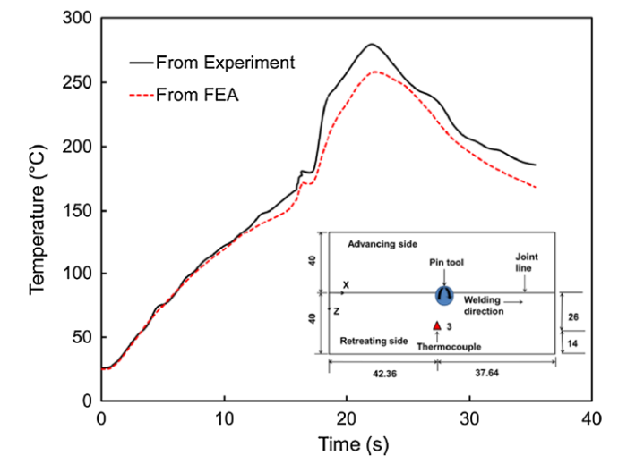
Figures 9 and 10 show the time histories of the temperature on the top surface at thermocouple location 3 (x = 42.36 mm, z = 26 mm) along the weld direction for two different weld schedules. The comparison shows that result from FEA analysis is in good agreement with experimental data and also shows a similar temperature profile. From the temperature profile, it can be seen that as the time progresses there is a swift increase in temperature when the pintool moves close to the thermocouple. The maximum temperature takes place at the top surface of the workpiece underneath the pintool shoulder as shown in Fig. 11. After the temperature reaches its peak value, it starts decreasing as the pintool moves farther away from the thermocouple. Based on these results, it can be said that the simulation profiles are close to the experimental profiles at the starting of welding. As the weld progresses forward, there is a small divergence of FEA profile from the experimental profile as the temperature profile reaches its peak temperature. This small deviation in temperature profile continues after the experimental profile reaches its peak temperature. This may be attributed to the fact that the simulation does not take into account the thermal properties of the pintool which was modeled as rigid element to avoid numerical complexities. Another reason for the observed deviation of numerical results may be that the thermal property of the workpiece is assumed to be temperature independent. Previous published work [21] has shown that using temperature-dependent properties for both pintool and workpiece provided better result.
Fig. 9 Temperature variation histories from experiment and FEA analysis at location 3 for Case-1 weld schedule
Fig. 10 Temperature variation histories from experiment and FEA analysis at location 3 for Case-2 weld schedule
Fig. 11 Temperature field from simulation (for Case-1 weld schedule)
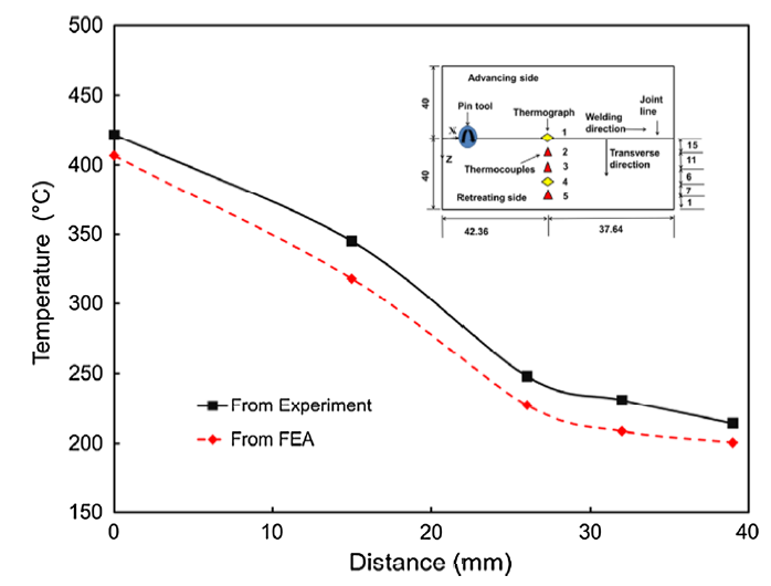
Figures 12 and 13 show the variation between FEA result and experimental results in the transverse direction of weld line. From both figures, it is obvious that experimental temperature profile is in close arrangement with the temperature from FEA analysis results as shown in Sect. 3.3. Also, Figs. 12 and 13 show that the temperature around the shoulder of the pintool is higher than adjoining location due to friction and plastic deformation. The maximum simulated temperatures in both cases were 406.74 and 450.6 °C for simulated Case-1 and Case-2 weld schedules, respectively. For both the weld schedule, the maximum temperature during welding is lower than melting temperature of AA2219-T87 (543 °C) [33], which is quite typical for FSW.
Fig. 12 Temperature variations along transverse direction between experimental and simulation data (for Case-1 weld schedule)
Fig. 13 Temperature variations along transverse direction between experimental and simulation data (for Case-2 weld schedule)
The error between experimentally recorded temperatures and FEA-simulated temperatures was calculated to quantify the deviation between the two temperatures at various distances perpendicular to the weld line. The error analysis between the experimental and the FEA temperature values is given in Tables 6 and 7. From these results, we can see that the absolute error is less than 4% for both weld schedules at the weld centerline. The results show that as the distance from the weld center increases, the absolute error slightly increases, but that the maximum absolute error is less than 10%. This may be due to the fact that the pintool was modeled as a rigid element where thermal properties are ignored. Also thermal properties of the workpiece were considered to be temperature independent, which may have caused small deviation between FEA analysis and temperature obtained from experiment. For both the weld schedules, the maximum absolute relative error is less than 10%, and the mean value of the error is below 7.08%.
Table 6 Error analysis for weld schedule Case-1 along transverse direction
| Distance from weld center (mm) | Temperature from FEA (°C) | Temperature from experiment (°C) | Absolute error (%) |
|---|---|---|---|
| 0 | 406.7 | 422 | 3.6 |
| 15 | 318.0 | 345 | 7.8 |
| 26 | 227.2 | 248 | 8.3 |
| 32 | 208.5 | 231 | 9.7 |
| 39 | 200.4 | 214 | 6.3 |
| Average error | 7.1 |
Table 7 Error analysis for weld schedule Case-2 along transverse direction
| Distance from weld center(mm) | Temperature from FEA (°C) | Temperature from experiment (°C) | Absolute error (%) |
|---|---|---|---|
| 0 | 450.5 | 458 | 1.6 |
| 15 | 335.1 | 364 | 7.9 |
| 26 | 257.6 | 280 | 8.0 |
| 32 | 228.5 | 251 | 8.9 |
| 39 | 208.2 | 228 | 8.6 |
| Average error | 7.0 |
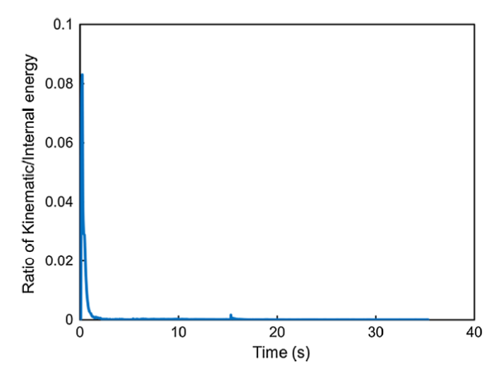
As mentioned in Sect. 2.6.4, mass scaling was used to reduce the computational costs in the current simulation. The ratio of kinematic energy and internal energy is analyzed to evaluate the effect of mass scaling as shown in Figs. 14 and 15 for both simulated weld schedules. Figures 14 and 15 show that the ratio is very small in the current simulations with a maximum ratio of less than 0.1. This represents that the FSW process is a quasi-static problem though both fixed and variable mass scales are used. Based on these results, it was concluded that the used mass scaling factor does not affect the numerical solutions of FSW significantly.
Fig. 14 Ratio of kinematic and internal energies with time for Case-1 weld schedule
Fig. 15 Ratio of kinematic and internal energies with time for Case-2 weld schedule
The heat produced during FSW causes the workpieces to join together. During the FSW, heat is generated through two possible ways, namely heat generation due to both friction between tool/workpiece and plastic deformation of the workpiece material. In the current study, both friction and plastic energy are studied by analyzing energy histories during FSW.
Table 8 lists the total plastic and frictional energies obtained from the FE simulations for the simulated weld schedules, i.e., Case-1 and Case-2. It can be seen that the friction work between tool and workpiece contributes the majority of the energy to the welding process. The frictional energy contributes the majority of the total energy which is about 90.8 and 88.6% for Case-1 and Case-2, respectively. The high rotational speed and the pintool pressure cause this high percentage of heat production due to differential velocity (slip rate) on the workpiece surface. As given in Table 8, the plastic energies obtained from the model are about 9.4 and 11.4% of the total energy dissipated for Case-1 and Case-2, respectively. These percentages are in the similar ranges compared to the values described by Bastier et al. [36]. Bastier et al. [36] reported that the contribution from plastic heat energy is only 4.4% of the total heat energy of FSW aluminum alloy, while the residual 95.6% heat energy being produced due to friction.
Table 8 Plastic/total energy ratio of different weld schedules
| Weld schedule | Rotational speed, \(N\)(rpm) | Weld speed, v (mm/s) | Total friction energy (J) | Total plastic energy (J) | Total energy (J) | \(\frac{{{\text{Total}}\,{\text{plastic}}\,{\text{energy}}}}{{{\text{Total }}\,{\text{energy}}}}\times\) 100% |
|---|---|---|---|---|---|---|
| Case-1 | 350 | 1.27 | 4.62 × 10⁴ | 4.76 × 10³ | 5.09 × 10⁴ | 9.4% |
| Case-2 | 350 | 2.54 | 4.92 × 10⁴ | 6.30 × 10³ | 5.55 × 10⁴ | 11.4% |
In the following sections, parametric studies are conducted to study the effects of rotational speed, travel speed, and plunge rate heat generation due to friction and plastic energy.
Various rotational speeds have been analyzed in a parametric study to investigate its influence on energy generation. Three different rotational speeds, namely 200, 350, and 450 rpm, were consideration. A fixed weld speed of v = 1.27 mm/s and a steady plunge rate of 0.4 mm/s have been used in the analysis.
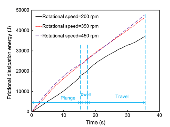
Figures 16 and 17 represent frictional dissipation energy and plastic dissipation histories, respectively. Based on these results, it is clear that higher dissipation energy is produced with higher rotational speeds. Figure 16 shows that the frictional dissipation energy increases almost linearly for different rotational speeds. Furthermore, frictional dissipation energy generated for rotational speed of 350 and 450 rpm is quite close. The amount of frictional heat energy generated for 200 rpm is low compared to 350 and 450 rpm. Experiments conducted by this research group have shown that this inadequate temperature promotes the development of defects like wormholes or internal cavities and trenching or surface cavities [29]. The increase in total frictional dissipation energy is about 19.9% as spindle rotational speed is raised from 200 to 350 rpm. Moreover, as the rotational speed is increased from 350 rpm to 450 rpm, the overall frictional energy increased about 3.0%. At high rotational speed, the high relative velocity of the material causes this high energy production. Figure 17 shows that the plastic dissipation energy increases sharply until the completion of the plunge stage for rotational speeds 350 and 450 rpm. After the plunge stage, there is linear increase in plastic energy dissipation. This can be explained by the fact that during plunge stage there is large amount of material penetrated by the pin nib (apex of the pintool) which causes high plastic deformation underneath the pintool. At the end of plungestage, plastic deformation becomes linear during dwell and travel stages as high deformations due to the compounded effect of plunging and stirring no longer exist. However, a similarly clear trend is not observed for the rotational speed of 200 rpm plastic dissipation energy profile, for which a sharp increase in plastic deformation during the plunge stage was not observed. Experiments by this research group have shown that this inadequate lack of plastic deformation promotes the development of defects like incomplete penetration which is classified as cold welds [29]. The amount of frictional heat energy generated for 200 rpm is also low compared to 350 and 450 rpm weld schedules. By increasing the rotational speed from 200 to 350 rpm, the total plastic heat energy dissipation increased is 68.1%, whereas increasing it from 350 to 450 rpm resulted in an increase in plastic heat energy of about 24.2%. Table 9 summarizes the effect of rotational speed on frictional and plastic dissipation energy. Table 9 shows that when the rotational speed increases, plastic dissipation energy increases considerably and the frictional dissipation energy increases only slightly. Similar results have been reported by Tang et al. [37] based on experimental work. Also, numerical simulations by Zhang et al. [18] and Awang et al. [38] have shown that higher rotational speed causes higher dissipation energy.
Fig. 16 Variation of frictional energy with rotational speed (plunge rate = 0.4 mm/s, v = 1.27 mm/s)
Fig. 17 Variation of plastic energy with rotational speed (plunge rate = 0.4 mm/s, v = 1.27 mm/s)
Table 9 Synopsis of energies for various rotational speeds
| Plunge rate (mm/s) | Rotational speed, \(N{ }\)(rpm) | Weld speed, v(mm/s) | Total frictional energy (J) | Change in frictional energya | Total plastic energy (J) | Change in plastic energya | Total energy | \(\left( {\frac{\text{Total plastic energy}}{\text{Total energy}}} \right)\times\) 100% |
|---|---|---|---|---|---|---|---|---|
| 0.4 | 450 | 1.27 | 4.76 × 10⁴ | 3.0% | 5.91 × 10³ | 24.2% | 5.35 × 10⁴ | 11.04% |
| 0.4 | 350 | 1.27 | 4.62 × 10⁴ | Base1 | 4.76 × 10³ | Base1 | 5.09 × 10⁴ | 9.35% |
| 0.4 | 200 | 1.27 | 3.70 × 10⁴ | 19.9% | 1.52 × 10³ | 68.1% | 3.85 × 10⁴ | 3.94% |
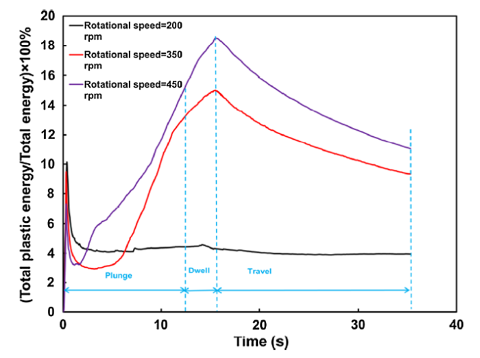
Figure 18 represents the variation of ratio of plastic energy to the total energy, (\(\frac{{{\text{Total}}\,{\text{plastic}}\,{\text{energy}}}}{{{\text{Total }}\,{\text{energy}}}}\)) with time for different rotational speeds. As the plunge stage starts (around 0.304 s when the contact between the pintool and the workpiece first occurs), there is a sudden rise in the plastic energy ratio for all rotational speed as the pin nib starts penetrating the workpiece followed by drop until the shoulder becomes in contact with the workpiece surface. Once the shoulder starts stirring the workpiece material, a second rise in the plastic energy ratio is observed, which is more pronounced for \(N =\) 350 rpm and \(N =\) 450 rpm during the plunge and dwell stages, but not as much for \(N =\) 200 rpm. During the plunge and dwell stages, the pin nib first perforates into the workpiece and then the pintool keeps on rotating in the same location, respectively, which causes large plastic deformations in the workpiece material. This high plastic deformation is what allows FSW to create a suitable weld joint. For weld schedules that produce low plastic deformations, e.g., \(N =\) 200 rpm, no such rise in energy ratio is observed during the plunge or dwell stage. Consequently, the insufficient plastic deformation eventually causes cold welds that typically result in weld defects as observed by our research group’s experimental work [29]. During the travel stage, the plastic energy ratio starts declining for all rotational speed. This indicates lower plastic deformation during the travel stage of FSW in comparison with the plunge and dwell stages. Finally, it is clear from the results in Table 9 that the weld schedule with \(N =\) 450 results in a higher energy ratio compared to other weld schedules due to the fact that higher rotational speeds cause more material to be deformed through plastic deformation.
Fig. 18 Variation of \(\frac{{{\text{Total}}\,{\text{plastic}}\,{\text{energy}}}}{{{\text{Total}}\,{\text{energy}}}}\) with time for different rotational speeds (plunge rate = 0.4 mm/s, v = 1.27 mm/s)
The influence of pintool weld speed on energy production during FSW was also investigated by considering three weld speeds 1.27, 1.69, and 2.54 mm/s. A fixed rotational speed of \(N\) = 350 rpm has been used in these analyses.
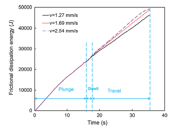
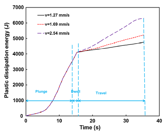
From, it can be seen that frictional dissipation energy rises as the welding speed increases. For different weld speeds, frictional dissipation energy is the same during the plunge stage, which is expected as there is no variation of weld speed during the plunge stage, i.e., all weld schedules have the same plunge rate and rotational speed. After the plunge stage, frictional dissipation energy for different weld speeds shows small variation with respect to time. Earlier work reported by Aziz et al. [21] also shows a similar behavior. Plastic dissipation energy profile shows similar behavior as frictional dissipation energy profile. After the plunge stage, plastic energy increases linearly with the increase in weld speed. The overall frictional energy rises about 5.3% when the weld speed is increased from 1.27 to 1.69 mm/s. Besides, the overall frictional energy increased about 0.8% when the weld speed is raised from 1.69 to 2.54 mm/s. Furthermore, when weld speed is increased from 1.27 to 1.69 mm/s, overall plastic dissipation energy is increased about 8.8%. Also as the welding speed increases from 1.69 to 2.54 mm/s, plastic dissipation energy increases about 20.7%. Table 10 summarizes the influence of weld speed on frictional and plastic energy, which shows that when the travel speed increases, the plastic dissipation energy increases significantly and the frictional dissipation energy increases marginally. The higher weld speed of the pintool results in faster time to rotate the workpiece material, which causes an increase in the production of local heat. Similar result has been reported by Zhang et al. [17] (Figs 19 and 20).
Table 10 Synopsis of energies for various weld speeds
| Plunge rate (mm/s) | Rotational speed, \({ }N{ }\)(rpm) | Weld speed, v(mm/s) | Total friction energy (J) | Change in frictional energyb | Total plastic energy (J) | Change in plastic energyb | Total energy | \(\left( {\frac{{{\text{Total}}\,{\text{plastic}}\,{\text{energy}}}}{{{\text{Total }}\,{\text{energy}}}}} \right)\times\) 100% |
|---|---|---|---|---|---|---|---|---|
| 0.4 | 350 | 2.54 | 4.92 × 10⁴ | 0.8% | 6.30 × 10³ | 20.7% | 5.55 × 10⁴ | 11.35% |
| 0.4 | 350 | 1.69 | 4.88 × 10⁴ | Base2 | 5.22 × 10³ | Base2 | 5.40 × 10⁴ | 9.66% |
| 0.4 | 350 | 1.27 | 4.62 × 10⁴ | 5.3% | 4.76 × 10³ | 8.8% | 5.09 × 10⁴ | 9.35% |
Fig. 19 Variation of frictional dissipation energy with welding speed (\(N\) = 350 rpm, plunge rate = 0.4 mm/s)
Fig. 20 Variation of plastic dissipation energy with welding speed (\(N\) = 350 rpm, plunge rate = 0.4 mm/s)
Figure 21 shows variation of energy ratio with time for different welding speeds. As discussed earlier, the behavior during the plunge and dwell stages can be summarized in an abrupt rise in the plastic energy ratio during the initial plunge stage (around 0.304 s) corresponding to the start of pin nib penetration into the workpiece. A drop in the plastic energy ratio after the initial rise is observed until the shoulder becomes in contact with the workpiece followed by a continuing increase in the plastic energy ratio during the remainder of plunge and dwell stages. Finally, a gradual decline in the plastic energy ratio during the travel stage is observed for all welding speed. This implies that the plate material undergoes lower plastic deformations during travel stage of FSW compared to plunge and dwell stages. The rate of decline in plastic energy ratio differs based on the travel speed of the weld schedule. Table 10 shows that the weld schedule with \(v =\) 2.54 mm/s produced a higher plastic energy ratio compared to other weld schedules as higher weld speed results in stirring more material along the path of the pintool, hence increasing plastic deformations.
Fig. 21 Variation of \(\frac{{{\text{Total}}\,{\text{plastic}}\,{\text{energy}}}}{{{\text{Total }}\,{\text{energy}}}}\) with welding speed (\(N\) = 350 rpm, plunge rate = 0.4 mm/s)
The last parameter investigated in this work was the plunge rate. Various plunge rates of 0.3, 0.4, and 0.6 mm/s were considered. The weld speed was kept fixed at 1.27 mm/s and spindle rotational speed was also fixed at 350 rpm during these simulations. The weld tool plunge depth was also fixed at 6.08 mm.
Figures 22 and 23 show the friction and plastic dissipation energy of simulation for all three considered plunge rates, respectively. Based on the plots, the energy increases with the decrease in plunge rate. A lower plunge rate allows more time to rotate the workpiece material and therefore generate more energy. The overall frictional energy increased 28.0% when the plunge rate is decreased from 0.6 to 0.4 mm/s. In the same manner, frictional energy increased 24.6% when the plunge rate is decreased from 0.4 to 0.3 mm/s. The plastic dissipation energy also follows the same trend observed for frictional dissipation energy. The slower the penetration speed, the higher the plastic dissipation energy. The overall plastic dissipation energy increased 28.5% when the plunge rate is decreased from 0.6 to 0.4 mm/s and increased 37.2% when the plunge rate is decreased from 0.4 to 0.3 mm/s.
Fig. 22 Variation of frictional energy with plunge rate (welding speed = 1.27 mm/s, \(N\) = 350 rpm)
Fig. 23 Variation of plastic energy with plunge rate (welding speed = 1.27 mm/s, \(N\) = 350 rpm)
Table 11 summarizes the plunge force influence on frictional and plastic energies. Comparable results have been mentioned in the work of Awang et al. [38].
Table 11 Synopsis of energies for various plunge rates
| Plunge rate (mm/s) | Rotational speed, \(N\)(rpm) | Weld speed, v (mm/s) | Total friction energy (J) | Change in frictional energyc | Total plastic energy (J) | Change in plastic energyc | Total energy | \(\frac{\text{Total plastic energy}}{\text{Total energy}}\times\) 100% |
|---|---|---|---|---|---|---|---|---|
| 0.3 | 350 | 1.27 | 2.89 × 10⁴ | 24.6% | 5.53 × 10³ | 37.2% | 3.44 × 10⁴ | 16.07% |
| 0.4 | 350 | 1.27 | 2.32 × 10⁴ | Base3 | 4.03 × 10³ | Base3 | 2.72 × 10⁴ | 14.81% |
| 0.6 | 350 | 1.27 | 1.67 × 10⁴ | 28.0% | 2.88 × 10³ | 28.5% | 1.95 × 10⁴ | 14.76% |
c with respect to Base3 weld schedule
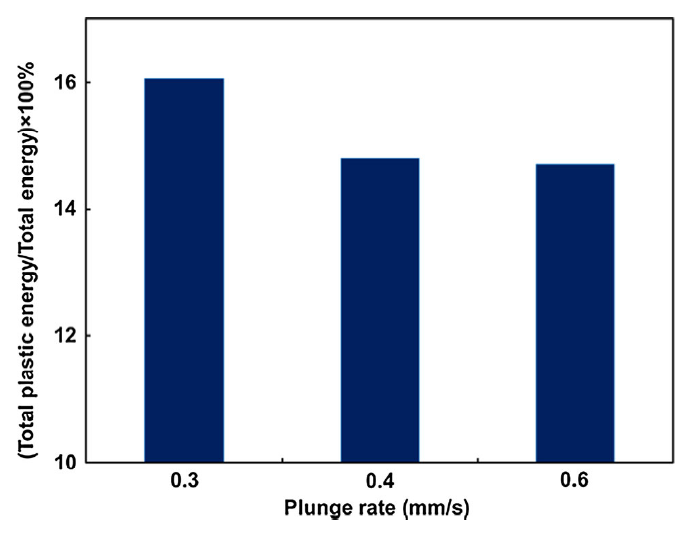
Figure 24 shows the effect of various plunge rates on the plastic energy ratio at the end of plunge stage. It can be seen that the weld schedule with a plunge rate of 0.3 mm/s results in a higher plastic energy ratio compared to the other two considered cases with plunge rates equal to 0.4 and 0.6 mm/s. This demonstrates that a slower plunge rate enables more time to rotate the workpiece material and therefore generate more plastic energy.
Fig. 24 Effect of plunge rate on plastic energy ratio at the end of plunge stage (welding speed = 1.27 mm/s, \(N\) = 350 rpm)
A fully coupled thermomechanical 3D finite element (FE) model has been developed to analyze thermal heat generation and distribution during friction stir welding. In this study, both heat dissipation from friction and plastic deformation are considered. The results obtained are summarized as follows:
1. Temperature field obtained from the FE simulations is similar to the temperature field obtained experimentally. Two separate weld schedules temperatures were investigated for comparing the experimental result with the result from the numerical simulation. For all cases considered, comparison from both weld schedules, the maximum relative error is lower than 10%, having a mean value of 7.1%.
2. Heat produced by friction between the pintool and workpiece produces majority of the energy (about 90.8% for Case-1 and 88.6% for Case-2 weld schedule).
3. Investigation was performed to study the influence of different weld process parameters—rotational speed, weld speed, and plunge rate. This study revealed that:
a. High rotational speed causes higher amount of frictional and plastic dissipation energies. Frictional dissipation energy behaves almost linearly with respect to time for different rotational speeds investigated. Plastic energy dissipation energy increases sharply during the plunge stage. Low rotational speed causes inadequate temperature due to the low frictional and plastic dissipation energies which eventually causes defects such as wormholes, surface cavities, and incomplete penetration.
b. Higher weld speeds cause more total frictional and plastic dissipation energies. However, it was found that friction dissipation energy and plastic dissipation energy remain the same during the plunge stage for different weld speeds. After the plunge stage, the frictional energy for different weld speeds shows small variation with respect to time.
c. At plunge and dwell stages of FSW, energy ratio (\(\frac{{{\text{Total}}\,{\text{plastic}}\,{\text{energy}}}}{{{\text{Total }}\,{\text{energy}}}}\)) increases as the time progresses. Throughout travel stage, a decline in the energy ratio is observed.
d. During plunge stage, a lower plunge rate causes higher friction and plastic dissipation energy.
e. When rotational speed and weld speed are increased, plastic dissipation energy increased significantly. The corresponding increase in the frictional dissipation energy under the similar conditions is shown to be minimal.
The authors have declared that no competing interests exist.

 WeChat
/
| 〈 |
|
〉 |


