Search for articles:
Zhao Zhang , Zhi-Jun Tan
Corresponding authors:
Received: 2019-03-22
Revised: 2019-05-17
Online: 2020-01-10
Copyright: 2020 Editorial board of Acta Metallurgica Sinica(English Letters) Copyright reserved, Editorial board of Acta Metallurgica Sinica(English Letters)
More
Abstract
Friction stir additive manufacturing is a newly developed solid-state additive manufacturing technology. The material in the stirring zone can be re-stirred and reheated, and mechanical properties can be changed along the building direction. An integrated model is developed to investigate the internal relations of process, microstructure and mechanical properties. Moving heat source model is used to simulate the friction stir additive manufacturing process to obtain the temperature histories, which are used in the following microstructural simulations. Monte Carlo method is used for simulation of recrystallization and grain growth. Precipitate evolution model is used for calculation of precipitate size distributions. Mechanical property is then predicted. Experiments are used for validation of the predicted grains and hardness. Results indicate that the average grain sizes on different layers depend on the temperature in stirring and re-stirring processes. With the increase in building height, average grain size is decreased and hardness is increased. The increase in layer thickness can lead to temperature decrease in reheating and re-stirring processes and then lead to the decrease in average grain size and increase of hardness in stir zone.
Keywords:
Friction stir additive manufacturing (FSAM) is an emerging additive manufacturing technology in recent years. FSAM originates from friction stir welding (FSW) and their fundamentals are similar. However, FSAM is used as additive manufacturing process, which results in reheating and re-stirring. In FSAM, the workpiece is built layer by layer in building direction. Different from overlap FSW, re-stirring and reheating times can be designed for controlling mechanical properties and microstructures. The rotating tool with a long pin (longer than the thickness of one built layer) leads to material flows and ensure that different layers can be joined together by FSAM. FSW has been successfully applied to joining of aluminum alloys [1, 2], magnesium alloys [3], titanium alloys [4, 5] and steels [6, 7]. In comparison with laser additive manufacturing, there are many advantages of FSW/FSAM such as no melt, no pollution and low distortions [8].
Li et al. [9] fabricated a Ti3Alp/Ti-6Al-4V surface layer via additive friction stir processing to investigate the formation mechanism and strengthening effect of the layer. FSAM was used by Mao et al. [10] for the study of mechanical properties and microstructures. It was found that different grain sizes exist along the build direction. The tensile strength of all the slices increases and the elongation decreases slightly in comparison to Al substrate. A multilayered stack of Mg-based WE43 alloy was built by FSAM by Palanivel et al. [11]. The strength of specimen after manufacturing is obviously higher than base material due to aging in FSAM. Through the FSAM manufacturing process, the hardness of magnesium alloy is increased from 97 HV (base material) to 120 HV, and the hardness of aluminum alloy is increased from 88 HV (base material) to 104 HV. This phenomenon illustrates the fact that FSAM is a high-performance route [12].
In the process of FSAM, reheating and re-stirring exist. This is a special feature which is different from that for FSW. The reheating and re-stirring can affect the microstructural evolutions and then mechanical properties. There are many numerical methods for simulation of microstructural evolutions, including Monte Carlo (MC) method [13], cellular automaton (CA) method [14] and phase field (PF) method [15]. Physical meaning in Monte Carlo model, as well as cellular automaton model, should be defined for simulation of recrystallization and grain growth in FSAM/FSW. Zhang et al. [16] further considered the effects of precipitates on grain growth and extended the Monte Carlo model to 3D case.
The Kampmann-Wanger numerical (KWN) model can be utilized for non-isothermal heat treatments [17]. This provides the possibility of application in welding simulations. Generally, the precipitate evolution is assumed to be determined by thermal history [18]. For Al-Mg-Si alloy (6xxx), the precipitate evolution is SSSS (supersaturated solid solution)-atomic clusters → G.P. zones → β″ (Mg5Si3) → β′ (Mg5Si3) → β (Mg2Si) [19]. It has been successfully applied to FSW for predictions of precipitates and mechanical properties.
The temperature can affect both the grain growth and the precipitate evolutions in FSAM. Different volume fractions of precipitates have various effects on grain coarsening speeds, which leads to different microstructures in stir zone (SZ) according to Wu and Zhang [20]. This means that it is possible to integrate different models together for the studies of internal relations from process parameters to microstructures and finally mechanical properties in FSAM. So, an integrated numerical model of FSAM is established in current work for investigation on process-microstructure-property relations. Experiments are carried out to verify the feasibility of established integrated model. The mechanism on the formation of different microstructures and mechanical properties is then studied.
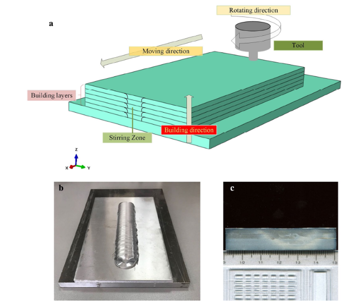
The schematic diagram of FSAM is shown in Fig. 1a. The specimens of FSAM are obtained by FSW machine. Infrared radiation thermometer (IRT) was used for process monitoring of temperature. A H13 steel tool was selected with a 24-mm-diameter shoulder. The pin length of welding tool was 8 mm, greater than the thickness of the building layer. The diameters of the conical pin ranged from 6 mm on the bottom to 8 mm on the top of the pin. In the experiment, the rotation speed of welding tool is 1000 rev/min and the transverse speed is 100 mm/min. AA6061-T6 was selected as the material for FSAM, and AA-6082 was utilized as a substrate. The sizes of building layer in FSAM were 200 mm × 110 mm × 4 mm, and the sizes of substrate were 250 mm × 150 mm × 8 mm.
Fig. 1 a Schematic diagram of FSAM, b specimen after FSAM, c 2-layer specimen after etching
The obtained specimens were cut and polished and then immersed in Keller reagent for 300 s. In our numerical model, the grain orientation is random; in the experiment, it is also random. In fact, what we need from experiment is only average grain size. This information can be easily obtained from scanning electron microscopy (SEM). So, the corroded samples were observed under SEM to obtain the average grain size. Vickers hardness tester (VHT) was used for the measurement of hardness distributions on the cross section of FSAM.
FSAM specimen is shown in Fig. 1b, c. The VHT area is about 7.5 μm × 7.5 μm. However, the measured area by transmission electron microscopy (TEM) for the precipitate size is about 200 nm × 200 nm [21, 22, 23]. The used precipitate evolution model is, in fact, a macro scale instead of a microscale (nanoscale) model. It is not a model for observation of precipitates. The different scales between the current model and the TEM lead to difficulties in direct comparison. However, the final hardness data, which is also the key point we are studying in this work, can be validated by direct comparison between experimental and numerical results.
The finite element model of FSAM is shown in Fig. 2. The building thicknesses are selected to be 2 mm, 4 mm and 6 mm, respectively. Moving heat source model [24, 25] is used for simulation of temperature rises in the FSAM process.
Fig. 2 Finite element models of FSAM with different building layer thicknesses: a 2 mm, case 1, b 4 mm, case 2, c 6 mm, case 3
The generated heat mainly comes from friction between the welding tool and the plate. It is replaced by a moving heat source. In Ref. [26], when the rotation speed of pin is changed from 500 to 1000 rpm, the heat generation of tool is approximately proportional to the rotation speed. The heat source is simplified to be a surface heat input [27, 28],
$P_{\text{s}} = \eta \frac{2}{3}\pi \mu p\omega \left( {r_{\text{s}}^{3} + 3l_{\text{p}} r_{\text{p}}^{2} } \right),$ (1)
where η is the heat fraction flowing into welding plate on tool-plate contact surface and is taken as 0.39 according to Nandan et al. [29], μ is frictional coefficient and is taken as 0.5 [30], P is the contact pressure along axial direction, which is lower than the actual flow stress of the material at the working temperature [31], ω is the rotational speed and lp is the length of pin.
In each numerical case, the length of the pin is greater than the thickness of one layer and slightly less than two layers in order to ensure an effective connection between two added layers. rs and rp are radii of shoulder and pin and are 12 mm and 4 mm, respectively. Birth-death element strategy is used for simulation of the building layers. The generation of total heat consists of two parts: the friction between the shoulder and the workpiece as well as the friction between the pin and the workpiece. The total heat input, including the contributions from the two mentioned heat generation aspects, is calculated according to Ref. [28]. Then, the total heat input power is expressed as a surface heat source. The spatial distribution of heat flux during friction stir welding follows the regularity found in Ref. [32].
The material’s physical and thermal properties are considered to be functions of temperature as shown in Ref. [27]. According to Chen et al. [33], different boundary conditions yield similar predictions on temperature. Convective boundary condition is selected,
$k\frac{\partial T}{\partial n} = h\left( {T - T_{\text{a}} } \right),$ (2)
where k is the thermal conductivity, h is the convection coefficient and Ta is the ambient temperature. AA6082 shows similar thermal physical data with AA6061-T6, as shown in Refs. [27, 34]. Moreover, the observation of cross section of experimental specimen shows the material on substrate does not enter the build layers. So, the selection of material parameters can hardly affect the numerical results from building layers.
The thermal process in FSAM is simulated using the heat transfer model. The governing equation for the transient heat transfer is given as,
${C\dot{T}} + {KT} = {P},$ (3)
where C is heat capacity matrix, K is heat conduction matrix and P is temperature load matrix. When the new layer is built, the elements for this layer are activated in numerical model. Then, the newly activated elements need to be considered in the heat capacity matrix, heat conduction matrix and temperature load matrix shown in Eq. (3) for finite element model of heat transfer.
MC model and KWN model are integrated for simulations of microstructural evolutions and mechanical properties. The flowchart for the proposed integrated model is shown in Fig. 3. The KWN model can be used to calculate the volume fraction of the precipitates and mechanical properties of the joint. Precipitates can hinder the grain boundary immigrations and the grain growth rates. Different volume fractions of precipitation have different effects on grain coarsening speeds in the SZ according to Ref. [20]. The calculated volume fraction of precipitate can be applied to the MC model for more accurate prediction of grain morphology.
Fig. 3 Flowchart for integrated model
The precipitate evolution model is widely used for precipitate calculation and prediction of mechanical properties of aluminum alloys, as shown in Refs. [17, 18, 35, 36]. This model is also adopted here for the simulation of the precipitate evolution in FSAM. With experimental validation, this model shows its success and advantages for the prediction of the mechanical properties of FSAM specimens. The nucleation rate for precipitate in FSAM can be written as [17, 18, 35, 36],
$j = j_{0} \exp \left[ { - \left( {\frac{{A_{0} }}{RT}} \right)^{3} \left( {\frac{1}{{\ln \left( {\bar{C} /C_{\text{e}} } \right)}}} \right)^{2} } \right]\exp \left( { - \frac{{Q_{\text{d}} }}{RT}} \right),$ (4)
where j0 is a material coefficient, which is the pre-exponential term to the nucleation rate j. A0 is a parameter related to the energy barrier for nucleation. $\bar{C}$(wt%) is the current mean concentration of Mg in matrix. Ce (wt%) is the equilibrium solute concentration at the precipitate/matrix interface. Qd (J mol-1) is the diffusion activation energy of element Mg in aluminum matrix, assuming that Mg is controlling the growth or dissolution of precipitation. R is the universal molar gas constant.
The equilibrium solute concentration of Mg at the precipitate/matrix interface is shown as follows:
$C_{\text{e}} = C_{\text{s}} { \exp }\left( { - \frac{{Q_{\text{s}} }}{RT}} \right),$ (5)
where Cs is pre-exponential term in simplified expression for Mg equilibrium concentration. Qs is the solvus boundary enthalpy.
According to the Gibbs-Thomson equation, equilibrium solute concentration of Mg at the precipitate/matrix interface Ci can be expressed as,
$C_{\text{i}} = C_{\text{e}} { \exp }\left( {\frac{{2\gamma V_{\text{m}} }}{rRT}} \right) ,$ (6)
where γ is the particle/matrix interfacial energy. Vm is the molar volume of precipitation. r is the particle radius.
When $\bar{C} = C_{\text{e}}$, the precipitates stop growing and the critical radius (rc) of the precipitated particles can be described as,
$r_{\text{c}} = \frac{{2\gamma V_{\text{m}} }}{RT}\left( {{ \ln }\left( {\frac{{\bar{C}}}{{C_{\text{e}} }}} \right)} \right)^{ - 1}.$ (7)
Then, a number density of j∆t nucleated particles is added during each time step, where the radius of a nucleated particle equals 1.05 rc. A new nucleated particle can grow if the radius is a little bit larger than the critical radius. The Mg solutes are either in the precipitates or the matrix of alloy. Its mass balance can be expressed as the following equation,
$\bar{C} = C_{0} - \left( {C_{\text{p}} - \bar{C}} \right)f ,$ (8)
where C0 is the initial concentration of Mg in aluminum alloy. Cp is the concentration of element inside the particle. f is the precipitate volume fraction.
The model for precipitates is discretized in radius direction. The volume fraction of precipitates is then calculated as,
$f = \frac{4}{3}\pi r_{i}^{3} N_{i} = {{\left( {C_{0} - \bar{C}} \right)} \mathord{\left/ {\vphantom {{\left( {C_{0} - \bar{C}} \right)} {\left( {C_{\text{p}} - \bar{C}} \right)}}} \right. \kern-0pt} {\left( {C_{\text{p}} - \bar{C}} \right)}},$ (9)
where Ni denotes the particle number. ri means the radius of ith particle.
The yield strength of the friction stir weld, σs, can be divided into three parts,
$\sigma_{\text{s}} = \sigma_{0} + \sigma_{\text{ss}} + \sigma_{\text{p}},$ (10)
where σss is the additional contribution from solid solution and σp from precipitates. σ0 is the intrinsic yield strength of pure aluminum.
The solute hardening due to the interstitials is computed by,
$\sigma_{\text{ss}} = \sum\limits_{i = 1}^{3} {k_{i} C_{i}^{2/3} },$ (11)
ki is the scaling factor for ith alloying element and Ci is its concentration. The solutes elements for solid solution are Mg, Si and Cu, indexed i = 1, 2 and 3. k1 = 66.3(MPa/wt%2/3), k2 = 29(MPa/wt%2/3) and k3 = 46.4(MPa/wt%2/3). The precipitate hardening is given by,
$\sigma_{\text{p}} = \frac{M}{{b\bar{r}}}\left( {2\beta Gb^{2} } \right)^{ - 1/2} \left( {\frac{3f}{2\pi }} \right)^{1/2} \left( {\frac{{\sum\limits_{i} {N_{i} F_{i} } }}{{\sum\limits_{i} {N_{i} } }}} \right)^{3/2} ,$ (12)
where β is a constant, Fi is the obstacle strength of the corresponding size in given discretized class and is related to the particle size. G is the shear modulus. b represents the Burgers vector. M is the Taylor factor. $\bar{r}$ is the mean particle radius. The calculation of Fi can be referred to by Myhr et al. [35]. The hardness is computed as follows,
$\text{HV} = 0.33\sigma_{\text{s}} + 16 .$ (13)
In MC model, a real square area in the SZ is represented by N × N lattice matrix. Each grid point is given a different number (1 - q) of grain orientations. The precipitation is given the orientation qi = q + 1. The law of energy calculation of each grid in integrated model is described as follows [37], and the precipitate is not included in the energy calculation,
$E = - J\sum\limits_{i = 1}^{m} { (\delta_{{q_{i} q_{j} }} - 1 )} ,$ (14)
where J is the grain boundary energy. δ is the Kronecker function.
In the process of FSAM, there is recrystallization in the SZ, and the nucleation rate related to strain rate is shown as follows [38]:
$\dot{n} = N_{0} \dot{\bar{\varepsilon }}{ \exp }\left( { - \frac{Q}{RT}} \right) ,$ (15)
where N0 is a constant and taken as 1024/s/m3. $\dot{\bar{\varepsilon }}$ is the equivalent strain rate.
In Ref. [26], when the rotation speed of pin is changed from 500 to 1500 rpm, the strain rate increases proportionally to the rotation speed. It is validated by experiments. The equivalent strain rate is calculated according to the size of pin and the rotating speed [26, 39, 40, 41],
$\mathop {\bar{\varepsilon }}\limits^{ \cdot } = \frac{{\omega \pi r_{\text{e}} }}{{L_{\text{e}} }},$ (16)
where re is represented by 0.78 of the radius of the SZ and Le is assumed to be the length of the pin. The recrystallization process and parameters of this equation were validated in Refs. [26, 39, 40, 41].
The formula that combines the Monte Carlo steps with time and temperature can be found in previous work [13],
$({\text{MCS}})^{{(n + 1)n_{1} }} = \left( {\frac{{L_{0} }}{{K_{1} l}}} \right)^{n + 1} + \frac{{(n + 1)\alpha C_{1}^{n} }}{{(K_{1} l)^{n + 1} }}\sum {\left[ {{ \exp }^{n} \left( { - \frac{Q}{{RT_{i} }}} \right)t_{i} } \right]} ,$ (17)
where K1 and n1 are constants, which are calculated according to trials and errors calculations. n is the ratio constant. l is the lattice length. α is a constant and is taken as 1.0. C1 can be described by the following equation,
$C_{1} = \frac{{2A\gamma ZV_{\text{m}}^{2} }}{{N_{\text{a}}^{2} h_{\text{P}} }}{ \exp }\left( {\frac{{\Delta S_{\text{f}} }}{R}} \right),$ (18)
where Na is the Avogadro’s number. hP is the Planck’s constant. ΔSf is the fusion entropy. Z is the average number per unit area.
The material parameters and constants in Eqs. (4-18) used for current simulation are summarized in Table 1 [13, 19, 37, 42].
Table 1 Material parameters and constants
| Physical property and value | |
|---|---|
| j | Nucleation rate (#/m3) |
| j0 | Material coefficient (3.07 × 1036) |
| A0 | Energy barrier for nucleation (18,000 J/mol) |
| R | Universal gas constant (8.314 J K-1 mol-1) |
| T | Temperature (K) |
| $\overline{C}$ | Mean concentration of Mg in matrix (wt%) |
| Ce | Equilibrium solute concentration of Mg at the precipitate/matrix interface (wt%) |
| Qd | Activation energy for diffusion (J/mol) |
| Cs | Pre-exponential term to Ce (290 wt%) |
| Qs | Activation energy for solvus boundary (41,000 J/mol) |
| Ci | Solute concentration at the particle/matrix interface (wt%) |
| Cp | Concentration of element inside the particle (wt%) |
| r | Particle radius (m) |
| γ | Particle/matrix interfacial energy (0.26 J/m2) |
| Vm | Molar volume of precipitation (7.62 × 10⁻⁵ m3/mol) |
| rc | Critical radius (m) |
| f | Volume fraction |
| Ni | Number of particles per unit volume within the size class ri (/m3) |
| σs | Yield strength (MPa) |
| σ0 | Intrinsic yield strength of pure aluminum (10 MPa) |
| σss | Contribution from alloying elements in solid solution to the overall macroscopic yield strength (MPa) |
| σp | Contribution from hardening precipitates to the overall macroscopic yield strength (MPa) |
| kMg | Scaling factor of Mg (66.3 MPa/wt%2/3) |
| kSi | Scaling factor of Si (29 MPa/wt%2/3) |
| kCu | Scaling factor of Cu (46.4 MPa/wt%2/3) |
| M | Taylor factor (3.1) |
| b | Magnitude of the Burgers vector (2.84 × 10⁻¹⁰) |
| $\overline{r}$ | Mean particle radius (nm) |
| β | Constant in expression for the dislocation line tension (0.36) |
| G | Shear modulus (2.7 × 10¹⁰ N/m3) |
| Fi | Interaction force between dislocations and particles within the size class ri (N) |
| m | Total number of sites near one lattice point (8) |
| N0 | Constant (1024/s/m3) |
| J | Lattice energy density |
| $\delta_{{q_{i} q_{j} }}$ | Kronecker delta function |
| re | Effective radius of SZ (0.007 m) |
| Le | Effective depth of SZ (0.008 m) |
| A | Accommodation probability (1) |
| Z | Average number per unit area (4.31 × 10²⁰ atoms/m2) |
| hP | Planck’s constant (6.624 × 10⁻³⁴ J s) |
| Vm | Atom molar volume (1.0 × 10⁻⁵ m3/mol) |
| $\Delta S_{\text{f}}$ | Fusion entropy (11.5 J/mol/K) |
| Na | Avogadro’s number (6.02 × 10²³/mol) |
| γ | Boundary energy (0.5 J/m2) |
| Q | Activation enthalpy (140,000 J/mol) |
| α | Ratio constant (1.0) |
| n | Ratio constant (0.1) |
The temperature field of the first layer in FSAM is measured by IRT system in the welding process, as shown in Fig. 4a. The change in surface smoothness caused by the formation of flash can have influences on observation figure by infrared thermometer. However, this is the most appropriate way to show both the peak value and distributions of temperatures, which provides validation for numerical model. The quantitative comparison of temperature in experiment and numerical model is shown in Fig. 4b. The maximum temperature of the 1st layer is 398.4 °C from experiment and is 390.7 °C in numerical model on the selected cross line. The error for peak temperature is 1.9%. The comparison shows the accuracy of the used process model of FSAM. This provides the basis for the following study of microstructure simulation and mechanical properties prediction.
Fig. 4 Temperature comparison between experiment and numerical model: a temperature in the 1st layer from IRT system, b comparison of temperature in the 1st layer
The effect of building thickness is then considered, as shown in Fig. 5. The maximum temperature occurs under the tool shoulder. The maximum temperature is 420.8 °C in case 1, 395.4 °C in case 2, and 380.9 °C in case 3. The increase in building thickness leads to a decrease in the maximum temperature.
Fig. 5 Temperature distribution of 1st layer for a case 1, b case 2, c case 3
The center point on the cross section is selected to show the temperature histories in case 1, as shown in Fig. 6. The maximum temperature on building layer is decreased with the increase in the building height. In case 1, the maximum temperature is 413.7 °C in 1st layer, 373.1 °C in 2nd layer, 362.1 °C in 3rd layer, 358.6 °C in 4th layer and 351 °C in 5th layer. Moreover, it can be seen that reheating for layers is a special feature for this solid-state additive manufacturing technology. The 1st layer is reheated for 4 times. The reheating peak temperature is 311.8 °C for 1st reheating, 184.8 °C for 2nd reheating, 158.8 °C for 3rd reheating and 137.5 °C for 4th reheating. The reheating peak temperature is gradually decreased. The 2nd layer is reheated for 3 times and the 3rd layer is reheated for 2 times and the 4th layer is reheated for 1 time.
Fig. 6 Numerical temperature-time histories of points in SZ in different layers: a 1st layer, b 2nd layer, c 3rd layer, d 4th layer, e 5th layer
The maximum temperature of center point is 413.7 °C, 380.9 °C and 363.9 °C corresponding in case 1, case 2 and case 3. With the increase in layer thickness, the maximum temperature and reheating peak temperature is decreased.
The increase in building height leads to a gradual decrease in the welding temperature of each layer. The temperature histories in Fig. 6 play an important role in the subsequent prediction of mechanical properties and evolution of microstructures. The peak temperatures of each added layer in heating and reheating processes are summarized in Tables 2, 3 and 4.
Table 2 Peak temperature of built layers in case 1 (°C)
| The 1st layer welded | The 2nd layer welded | The 3rd layer welded | The 4th layer welded | The 5th layer welded | |
|---|---|---|---|---|---|
| 1st layer | 413.772 | 311.842 | 184.893 | 157.761 | 137.457 |
| 2nd layer | - | 373.093 | 301.951 | 266.616 | 229.218 |
| 3rd layer | - | - | 362.107 | 304.659 | 262.476 |
| 4th layer | - | - | - | 358.635 | 299.035 |
| 5th layer | - | - | - | - | 350.793 |
Table 3 Peak temperature of built layers in case 2 (°C)
| The 1st layer welded | The 2nd layer welded | The 3rd layer welded | The 4th layer welded | The 5th layer welded | |
|---|---|---|---|---|---|
| 1st layer | 380.945 | 243.617 | 146.36 | 114.658 | 93.407 |
| 2nd layer | - | 345.433 | 246.809 | 187.875 | 149.408 |
| 3rd layer | - | - | 336.052 | 241.118 | 185.395 |
| 4th layer | - | - | - | 315.929 | 225.253 |
| 5th layer | - | - | - | - | 310.524 |
Table 4 Peak temperature of built layers in case 3 (°C)
| The 1st layer welded | The 2nd layer welded | The 3rd layer welded | The 4th layer welded | The 5th layer welded | |
|---|---|---|---|---|---|
| 1st layer | 363.945 | 210.844 | 115.749 | 86.5807 | 69.6053 |
| 2nd layer | - | 335.823 | 212.026 | 149.686 | 115.205 |
| 3rd layer | - | - | 321.065 | 209.375 | 149.501 |
| 4th layer | - | - | - | 311.498 | 204.751 |
| 5th layer | - | - | - | 300.105 |
The KWN model is utilized for analysis of the mechanism for controlling the variations in mechanical properties. The point in the SZ on the first layer of case 2 is selected for analysis. The particle number of precipitates (Mg2Si) decreases from 2.90073 e22/m3 in the base metal to 9.66246e20/m3 in the SZ at the peak temperature, as shown in Fig. 7. Then, Mg2Si is precipitated in the following cooling process and the particle number starts to increase to 1.10298e21/m3. The particle number of Mg2Si increases to 1.2148e21/m3 when the second layer is built. The increase in particle number becomes very small when the third, fourth and fifth layers are continuously built. At the same time, the mean radii of precipitates are changed in the additive manufacturing process. When the first layer is heated, the mean radius of precipitates increases from 4.62296 to 12.0113 nm. In the subsequent cooling process, the mean radius of precipitates is decreased to 10.9229 nm. With the temperature decrease, the new precipitates of Mg2Si can generate from the matrix. The radius of newly generated precipitates is very small. So, the average radius decreases.
Fig. 7 Variations in particle number and mean particle radius of precipitates
The numerical yield stress and hardness variation processes can be seen in Fig. 8. The particle number is the direct reason for the increase in mechanical property and the reheating process can produce the increase in particle number which is beneficial to the enhancement of the material. So, the hardness is 67.33 HV and the yield strength is 155.55 MPa when the first layer is built. When the second layer is added, the hardness of selected point is increased to 67.58 HV and the yield strength is increased to 156.29 MPa. The experimental hardness is 73 HV and the error is 7.4%. So, the predicted value can be fitted with the experimental one. The hardness and yield stress also have negligible increases when the third, fourth and fifth layers are added.
Fig. 8 Variations in yield stress and hardness
With the increase in building height, the maximum temperature of the SZ decreases, as shown in Fig. 6. It leads to a raise in hardness in the SZ on different layers. The numerical hardness rises from 63.46 HV on the first layer to 84.3 HV on the fifth layer in case 1 and from 67.58 HV to 97.86 HV in case 2 and from 74.44 HV to 104.13 HV in case 3 which is close to the hardness of the base metal. Figure 9 illustrates the variation of hardness on different layers in three cases. The smaller layer thickness can lead to softer materials in SZ.
Fig. 9 Variations in hardness of points in SZ in different layers
The MC model coupled with precipitate volume fractions can predict the microstructural evolution. Figure 10 shows the microstructure of the SZ after the second layer is built. Figure 10a, c shows experimental specimens observed by SEM. Figure 10b, d shows simulation results computed by MC model with precipitate effects. The mean grain size is measured according to ASTM linear intercept method [43]. The average grain size in the first layer of the SZ is 11.5 μm and in the second layer is 14.22 μm which are obtained by SEM images. The simulation results indicate that the average grain size in the first layer in the SZ is 10.62 μm and in the second layer is 15.05 μm. The errors are 7.6% and 5.8%, respectively. The predicted values can be fitted with the experimental ones. The average grain size in the first layer is smaller than that of second layer. The maximum temperature of first layer is higher than that of second layer. But when the second layer is added, the material in the first layer is re-stirred and reheated. The re-stirring leads to a new recrystallization. The recrystallization with lower reheating temperature is the real reason for the decrease in grain sizes in the first layer.
Fig. 10 Comparison of grains between experimental and numerical model: a first layer for 2-layers specimen, b first layer for 2-layers specimen, c second layer for 2-layers specimen, d second layer for 2-layers specimen
Figure 11 illustrates the average grain sizes in the SZ on different building layers in three cases. We calculated the average grain size of the four layers because the fifth layer has not experienced reheating and re-stirring processes. In case 1, the average grain size in the first layer of the SZ is 11.5 μm and decreases to 10.31 μm in the fourth layer. In case 2, the average grain size in the first layer of the SZ is 8.57 μm and decreases to 8.2 μm in the fourth layer. In case 3, the average grain size in the first layer of the SZ is 8.1 μm and decreases to 7.89 μm in the fourth layer. It is worth mentioning that the average grain size of the second layer is reduced to 7.89 μm. So, as the increase in building height, the average grain size of the SZ decreases. The smaller thickness of the building layers means the larger average grain size in the SZ.
Fig. 11 Average grain size in SZ in different layers
An integrated model of process-microstructure-property simulation is established for the study of FSAM. Corresponding experiments are conducted for validation. The results show that the numerical simulation results are in good agreement with the experimental results, which verifies the feasibility of the proposed integrated model.
1. Both the temperature of built layer and the temperature in reheating are decreased when the building height is increased. The increase in layer thickness leads to the decrease in temperature in FSAM.
2. The hardness, as well as yield strength, is increased with the increase in building height due to the decrease in reheating peak temperature. Smaller layer thickness leads to lower hardness and yield strength.
3. The grain morphologies are different in different building heights due to the different reheating temperatures. The increase in building height leads to the smaller average grain size in the SZ. The decrease in building thickness leads to the increase in average grain size.
This work was financially supported by the National Natural Science Foundation of China (No. 11572074).

 WeChat
/
| 〈 |
|
〉 |


