Search for articles:
Jiu-Zhou Zhao , Tauseef Ahmed
Corresponding authors:
Received: 2016-06-22
Revised: 2016-09-30
Online: 2017-01-20
Copyright: 2017 Editorial board of Acta Metallurgica Sinica(English Letters) Copyright reserved, Editorial board of Acta Metallurgica Sinica(English Letters)
More
Abstract
Immiscible alloys gained a considerable interest in last decades due to their valuable properties and potential applications. Many experimental and theoretical researches were carried out worldwide to investigate the solidification of immiscible alloys under the normal gravity and microgravity condition. The objective of this article is to review the research work in this field during the last few decades.
Keywords:
List of symbols
C Concentration (mole fraction)
Cm Mean field concentration in the liquid matrix (mole fraction)
Cd Concentration of the droplet (mole fraction)
C∞ Equilibrium composition at a flat interface boundary (mole fraction)
CB Concentration of solute in the matrix at the interphase boundary (mole fraction)
Cmix Concentration of the alloy (\( C_{\text{mix}} = \left( {1 - \phi } \right)C_{\text{m}} + \phi C_{\text{d}} \)) (mole fraction)
D Diffusion coefficient (m2/s)
DAB Diffusion coefficient of the solute A in the solvent B (m2/s)
DBB Self-diffusion coefficient of the solvent B (m2/s)
D Goldschmidt atomic diameter (m)
dA, dB Atomic diameter of the solute A and the solvent B (m)
dD Diameter of the droplet (m)
ez Unit vector in the z direction
er Unit vector in the radial direction r of the sample
F Free energy function
F Radius distribution function of the MPDs
G(A+B) Gibbs free energy of the two unmixed components A and B (J/mol)
Galloy Gibbs free energy of an alloy (J/mol)
\( G_{\text{A}}^{0} \), \( G_{\text{B}}^{0} \) Gibbs free energy of the pure component A and B (J/mol)
\( \Delta G_{\text{v}} \) Gain in free energy per unit volume on nucleation (J/m3)
\( \Delta G_{\text{c}} \) Energy barrier for nucleation (J)
g Acceleration due to gravity (m/s2)
h Planck constant (6.626 × 10⁻³⁴ J s)
\( \Delta H_{\text{mix}} \) Molar mixing enthalpy (J/mol)
ΔH0 Constant term related to the interatomic interaction (J/mol)
I Nucleation rate of the MPDs [nuclei/(m3 s)]
J Molar flux of solute from or to a particle/droplet [mol/(m2 s)]
JD Molar flux from or to a particle/droplet due to pure diffusion [mol/(m2 s)]
kB Boltzmann’s constant (1.3807 × 10⁻²³ J/K)
L1, L2 A-rich and B-rich liquid phases
M Atomic mass (amu)
NA Avogadro number (6.022 × 10²³/mol)
N0 Number density of atoms per unit volume (m-3)
N Number density of the MPDs (m-3)
R Radius of the minority phase droplet (m)
Rg Gas constant (8.31447 J/mol K)
R* Critical radius for the nucleation of the MPDs (m)
r Radial position in a cylindrical sample (m)
S Supersaturation (\( S = C_{m} - C_{\infty } \)) (mole fraction)
S′ Dimensionless supersaturation (\( \frac{{C_{\text{m}} - C_{\infty } }}{{C_{\text{d}} - C_{\infty } }} \))
S1, S2 Solid phase A and solid phase B
\( \Delta S_{\text{mix}} \) Molar mixing entropy (J/K)
T Absolute temperature (K)
TA, TB Melting temperature of the pure component A and B (K)
TC Critical temperature (K)
TM Monotectic temperature (K)
TE Eutectic temperature (K)
TW Wetting temperature (K)
Tm Melting temperature (K)
t Time (s)
∇T Temperature gradient (K/m)
u Droplet/particle moving velocity (m/s)
us Stokes velocity (m/s)
uM Marangoni velocity (m/s)
V Moving velocity of the matrix melt (V = V0 + Vc) (m/s)
V0 Solidification velocity (m/s)
VC Convective velocity (m/s)
XA, XB Molar or atomic fraction of the component A and B
\( x_{{{\text{L}}_{ 1} }} \), \( x_{{{\text{L}}_{2} }} \) Composition of the liquid phase L1 and L2
x Distance (m)
Greek symbols
σ L-L interfacial energy (J/m2)
Ω Molar volume (m3/mol)
\( \Omega _{\text{A}}^{{}} \), \( \Omega _{\text{B}}^{{}} \) Molar volume of the component A and B (m3/mol)
\( \Omega _{\text{d}} \)
Molar volume in the droplet (m3/mol)
η
Dynamic viscosity (Pa s)
\( \eta_{\text{m}}^{{}} \)
Viscosity of the matrix (Pa s)
\( \eta_{\text{d}} \)
Viscosity of the MPDs (Pa s)
\( \mu_{\text{A}} \), \( \mu_{\text{B}} \)
Chemical potentials of the component A and B (J/mol)
υ Kinematic viscosity (m2/s)
\( \rho_{\text{m}} \) Density of the matrix (kg/m3)
\( \rho_{\text{d}} \) Density of the MPDs (kg/m3)
\( \rho^{\text{mix}} \) Density of the alloy (kg/m3)
\( \lambda_{\text{m}} \) Thermal conductivity of the matrix [W/(K m)]
\( \lambda_{\text{d}} \) Thermal conductivity of the MPDs [W/(K m)]
\( \lambda_{{}}^{\text{mix}} \) Thermal conductivity of the alloy [W/(K m)]
Φ Phase field variable
ϕ Volume fraction of the MPDs
Immiscible alloys are characterized by the presence of a miscibility gap in their phase diagrams, as shown in Fig. 1. Many of them have great potential applications as structural and functional materials [1-4]. For example, Cu-Pb, Al-Pb and Al-Bi are advanced bearing materials for the automotive industry, if the soft Pb or Bi phase can be well dispersed in the hard matrix [5, 6]. Cu-Fe and Cu-Cr are high-strength and high electric conductive materials, and Cu-Co is excellent magnetoresistive material [7-9], etc. However, immiscible alloys have an essential drawback that the miscibility gap in the liquid state poses problems during solidification. When a homogenous single-phase liquid is cooled into the miscibility gap, the liquid-liquid (L-L) decomposition occurs [10]. Generally, the L-L decomposition starts with the nucleation of the minority phase liquid in the form of droplets (MPDs). These droplets then grow by the diffusion of solute in the matrix. They may also settle or float due to the density difference between the two liquids under the action of gravity (Stokes sedimentation) and migrate due to a temperature or concentration gradient (Marangoni motion). The Stokes and Marangoni motions of the droplets cause the formation of a phase-segregated microstructure in immiscible alloys [11]. In recent decades, plenty of efforts have been made to investigate the solidification behavior of immiscible alloys [12, 13]. Great progress has been made in this field. It has been demonstrated that some special techniques, such as powder metallurgy, strip casting, stir casting, centrifugal casting and rapid solidification, may have great potentials in the manufacturing of immiscible alloys with a well-dispersed microstructure [14-16]. Some of these techniques, e.g., centrifugal casting, have been employed in industry for the manufacturing of immiscible alloys [17, 18].
Fig. 1 Schematic phase diagram of an alloy with a miscibility gap in the liquid state
This article will review the research work on the solidification of immiscible alloys in the last few decades.
The components of an immiscible alloy are completely miscible in the liquid state above the binodal line temperature. Below the binodal line, two liquids L1 and L2 with different chemical compositions coexist in equilibrium. At temperature TM, the monotectic reaction (L1 → S1 + L2) takes place. At temperature TE, L2 solidifies through the eutectic reaction (L2 → S1 + S2).
The origin of the miscibility gap in the liquid state may be described as follows: At a given temperature and pressure, the molar Gibbs free energy of a system consisting of two unmixed liquid components is given by:
$$ G_{{({\text{A+B}})}} = X_{\text{A}} G_{\text{A}}^{0} + X_{\text{B}} G_{\text{B}}^{0} . $$ (1)
The molar Gibbs free energy of an alloy of composition XB is given by:
$$ G_{\text{alloy}} \, = \, X_{\text{A}} \mu_{\text{A}} + \, X_{\text{B}} \mu_{\text{B}} , $$ (2)
where \( \mu_{\text{A}} \) and \( \mu_{\text{B}} \) can be obtained by plotting the tangent to the Galloy versus concentration X curve at the point XB, as shown in Fig. 2.
Fig. 2 Change in Gibbs free energy on alloy formation
Alloy formation at composition XB results in a reduction in the Gibbs free energy, which can be written as:
$$ \Delta G_{\text{alloy}} \, = \, X_{\text{A}} \left( {\mu_{\text{A}} - G_{\text{A}}^{ 0} } \right) + \, X_{\text{B}} \left( {\mu_{\text{B}} - G_{\text{B}}^{0} } \right). $$ (3)
The molar Gibbs free energy of mixing is related to the molar mixing enthalpy \( \Delta H_{\text{mix}} \) and the molar mixing entropy \( \Delta S_{\text{mix}} \) as follows:
$$ \Delta G_{\text{alloy}} =\Delta H_{\text{mix}} - T\Delta S_{\text{mix}} . $$ (4)
The shape of the \( G_{\text{alloy}} - X \, \) curve depends upon the enthalpy and entropy terms. The entropy change on mixing stems from the change of ordering on alloy formation. In an ideal system, the atoms of the constituents are distributed randomly in the volume of the liquid alloy and the entropy of mixing is given by:
$$ \Delta S_{\text{ideal}} = - R_{\text{g}} [X_{\text{A}} \ln X_{\text{A}} + X_{\text{B}} \ln X_{\text{B}} ]. $$ (5)
The molar enthalpy of mixing is related to the A-B, A-A and B-B interatomic interactions. For simplicity, considering only the nearest neighbor interactions such as in the regular solution model, \( \Delta H_{\text{mix}} \) is given by:
$$ \Delta H_{\text{mix}} =\Delta H_{0} X_{\text{A}} X_{\text{B}} , $$ (6)
where ΔH0 is a constant term related to the interatomic interaction.
Depending on whether the interatomic interaction energy in the alloy is stronger or weaker than the unmixed components, there is a tendency for compound formation (preferred neighborhood of different atoms) or toward phase separation (preferred neighborhood of same atoms). Immiscible alloys are generally characterized by a positive enthalpy of mixing (\( \Delta H_{\text{mix}} \)), which means that the atomic size difference of the constituent elements is large and the electronegativity difference is small [19]. According to the Miedema’s model, the ΔH0 takes a positive value if the difference in the electron density parameters of the components is large and the difference in the electron work function of the components is small [20]. For a system with a positive ΔH0, the Gibbs free energy versus composition curve has a shape as shown in Fig. 3a at a sufficiently low temperature. The points a and b at the G-X curve have the same slope or common tangent, indicating that a homogenous liquid phase with composition XB tends to decompose into two liquids of the composition \( X_{\text{B}}^{ 1} \) and \( X_{\text{B}}^{ 2} \), respectively. This phase transformation leads to a reduction in the molar Gibbs free energy from G0 to G1. The T-X line defined by this common tangent is called the binodal line. Based on the fact that the chemical potentials of each component are equal in the phases in equilibrium, one can derive a simple relation between temperature and the composition of the coexisting phases within the miscibility gap for a regular solution:
$$ T = \frac{{\Delta H_{0} (1 - 2X_{\text{B}} )}}{{R_{\text{g}} (\ln X_{\text{A}} - \ln X_{\text{B}} )}}. $$ (7)
Fig. 3 a Variation of the liquid free energy at 900 K calculated with ΔH0 = 20 kJ/mol, b phase diagram showing the miscibility gap and spinodal line in a regular solution system [
With increasing temperature, the compositions \( X_{\text{B}}^{ 1} \) and \( X_{\text{B}}^{ 2} \) approach each other until both are equal at the critical temperature TC. For a regular solution, TC corresponds to a composition \( X_{\text{A}} = X_{\text{B}} = 0.5 \) and it increases with the interaction parameter (ΔH0):
$$ T_{\text{C}} = \frac{{\Delta H_{0} }}{{ 2R_{\text{g}} }}. $$ (8)
The loci of the points in the free energy curve where \( \frac{{\partial^{2} G}}{{\partial X^{2} }} = 0 \) give the spinodal boundary. For a regular solution, the spinodal line is described as:
$$ T_{\text{SP}} = \frac{{2\Delta H_{0} }}{{R_{\text{g}} }}X_{\text{A}} X_{\text{B}} . $$ (9)
A phase diagram showing a miscibility gap in the liquid state can be divided into three regions [21]: stable, metastable and unstable region, as shown in Fig. 3b. The liquid outside the miscibility gap is stable, and the corresponding solution is homogenous because any finite fluctuation in composition is accompanied by an increase in free energy. The liquid inside the spinodal line is unstable because any small fluctuation in composition that produces the A-rich and B-rich regions will cause a decrease in free energy and, thus, the L-L phase separation will occur spontaneously without any energy barrier. This is called the liquid-state spinodal decomposition. The region between the binodal and spinodal lines is metastable because a finite fluctuation in composition can be accompanied by a reduction in free energy although the liquid is stable against an infinitesimal composition fluctuation. Therefore, the phase separation into two liquids occurs by nucleation and growth and also there is an energy barrier to overcome.
Generally, the enthalpy and entropy of mixing depend on composition and temperature in a different way as in the regular solution. The deviation from the ideal behavior is expressed as the so-called excess quantities:
$$ \Delta G_{\text{excess}} =\Delta G -\Delta G_{\text{ideal}} , $$ (10)
$$ \Delta S_{\text{excess}} =\Delta S -\Delta S_{\text{ideal}} , $$ (11)
$$ \Delta H_{\text{excess}} =\Delta H -\Delta H_{\text{ideal}} , $$ (12)
where \( \Delta G_{\text{ideal}} \) is the free energy change for an ideal solution, \( \Delta S_{\text{ideal}} \) is the ideal entropy of mixing, and \( \Delta H_{\text{ideal}} \) is the enthalpy of mixing for ideal solution (\( \Delta H_{\text{ideal}} \, = \, 0 \)).
The thermodynamic properties can be expressed by the so-called Redlich-Kister ansatz [22]:
$$ \Delta H = \sum\limits_{i}^{{}} {A_{i} X_{\text{A}} X_{\text{B}} (X_{\text{A}} - X_{\text{B}} )} {}^{i}, $$ (13)
$$ \Delta S_{\text{excess}} = - \sum\limits_{i}^{{}} {B_{i} X_{\text{A}} X_{\text{B}} (X_{\text{A}} - X_{\text{B}} )} {}^{i}, $$ (14)
$$ \Delta G_{\text{excess}} = \sum\limits_{i}^{{}} {(A_{i} - TB_{i} )X_{\text{A}} X_{\text{B}} (X_{\text{A}} - X_{\text{B}} )} {}^{i}. $$ (15)
The coefficients Ai and Bi are determined from the measurements of the thermodynamic quantities and optimized to fit as close as possible to the measured shape of the binodal line. The values of coefficients Ai and Bi for a few binary systems are listed in Table 1.
Table 1 Coefficient sets for a few liquid binary alloy systems to express the Gibbs free energy
| System | i | Ai (J/mol) | Bi [J/(mol K)] | References |
|---|---|---|---|---|
| Al-Pb | 0 | 47,933.60 | -10.71995 | [19] |
| 1 | 14,407.33 | -6.65287 | ||
| 2 | 4742.36 | -0.72034 | ||
| Al-Bi | 0 | 24,649.18 | -3.04970 | [23] |
| 1 | 13,282.64 | -5.92753 | ||
| 2 | 18,519.75 | -12.33873 | ||
| 3 | 6959.30 | -2.24613 | ||
| Al-In | 0 | 18,641.14 | 1.74886 | [19] |
| 1 | 558.36 | 1.14350 | ||
| 2 | 10,692.88 | 7.47862 | ||
| 3 | 1346.56 | 0 | ||
| Cu-Fe | 0 | 35,625.8 | -2.19045 | [24] |
| 1 | 1529.8 | -1.15291 | ||
| 2 | 12,714.4 | -5.18624 |
Miscibility gaps can be divided into two types: (a) miscibility gap in the equilibrium liquid state (stable miscibility gap), e.g., Al-Pb and Bi-Zn systems and (b) miscibility gap in the metastable undercooled liquid state (metastable miscibility gap), e.g., Cu-Co and Cu-Cr systems. Considering that the liquidus is the boundary between the liquid phase region and the solid + liquid mixture region, the miscibility gap located above the liquidus line is stable, while the miscibility gap located below the liquidus is metastable.
The binodal lines in some systems are nearly symmetrical, and the critical concentration is close to the one for the regular solution, as for Ga-Hg and Al-Pb alloys. The phase diagrams of some alloys, such as Bi-Ga and Bi-Zn, show an asymmetrical miscibility gap, i.e., the binodal lines are not symmetrical and the critical concentration deviates from the one for the regular solution. A miscibility gap in the liquid state also exists in some systems that are composed of a transition metal (Ni, Fe, V, etc.) and a main group element (especially lower-melting-point elements such as Pb, Sn, In and Bi). Even the elements with similar chemical properties may show a miscibility gap in the liquid state, e.g., Na-Li system. Some alloys, e.g., Eu-Sc and Yb-Tb, show miscibility gap in the liquid state due to the difference in the electronic configurations of the constituent elements. Metastable miscibility gap may also appear in some systems consisting of two transition metals, such as Cu-Cr, Cu-Co and Cu-Fe.
The solidification process and microstructure of immiscible alloys are strongly dependent on the thermophysical properties, such as the L-L interfacial tension, diffusivity and viscosity.
An imbalance interatomic attractive force causes a higher potential energy of atoms at the interfacial region than in the bulk phase. This results in an excess free energy per unit area that is numerically equivalent to the interfacial tension [25]. The L-L interfacial tension and its temperature dependence are essential for understanding the microstructure evolution of immiscible alloys because it has a dominating effect on the nucleation, growth/coarsening and Marangoni motion of the MPDs during the L-L phase transformation [26, 27].
The measuring methods for the interfacial energy can basically be divided into static and dynamic ones. The measured data for the L-L interfacial energy in immiscible systems are scarce due to the experimental difficulties. Hoyer et al. [28-30] measured the L-L interfacial tension for Ga-Hg, Ga-Pb, Al-Bi, Al-In and Al-Pb immiscible systems in a wide temperature range. Recently, Kaban et al. [31-34] determined the L-L interfacial energies for binary, ternary and quaternary immiscible systems over a wide temperature and composition range. The experimental values of the L-L interfacial energies for some typical immiscible systems are listed in Table 2.
Table 2 Experimental values of the L-L interfacial energy for some typical immiscible systems at the monotectic temperature [
| System | Monotectic temperature Tm (K) | Critical temperature TC (K) | Interfacial tension σ (mJ/m2) |
|---|---|---|---|
| Al-Bi | 930 | 1310 | 56.7 |
| Al-In | 912 | 1110 | 25.5 |
| Al-Pb | 932 | 1695 | 125.5 |
The theoretical models [35-44] for the calculation of the L-L interfacial energy are based on either of the two concepts: One is presuming a sharp interface between the two phases which could be defined as a single atomic layer and calculate the energy of atomic pair traversing the interface and the other is recognizing the interface as a thin film and calculates the energy of the film-like phase which consists of three or more atomic layers. These two concepts are typically represented by the Becker model [35] and the Cahn-Hilliard model [36], respectively.
Immiscible system is considered as a regular solution in the Becker model, and the interfacial energy is given by [35]:
$$ \sigma = \frac{{N^{*} }}{{zN_{\text{A}} }}\Delta H_{0} \left( {x_{{{\text{L}}_{ 1} }} - x_{{{\text{L}}_{ 2} }} } \right)^{2} , $$ (16)
where N* is the number of atoms per unit interface area and z is the coordination number. For fluids, z ≈ 10. ΔH0 is related to the critical temperature as given in Eq. (8).
The interface is considered as an intermediate transition layer with a continuous change in concentration normal to the interface in the Cahn-Hilliard model, and the interfacial energy is given by [36]:
$$ \sigma = 2N_{0} \Upsilon k_{\text{B}} T_{\text{C}} (1 - T/T_{\text{C}} )^{ 1. 5} , $$ (17)
where N0 is the number of atoms per unit volume at the interface and Υ is the interaction distance. If the interactions other than those between the nearest neighbors are neglected, \( \Upsilon = {{r_{0} } \mathord{\left/ {\vphantom {{r_{0} } {\sqrt 3 }}} \right. \kern-0pt} {\sqrt 3 }} \). r0 is the intermolecular distance.
The exponential value of the Cahn-Hilliard model is very close to the model that is derived based on the renormalization theory of critical phenomenon [37, 38]:
$$ \sigma = \sigma_{0} (1 - T/T_{\text{C}} )^{ 1. 2 6} . $$ (18)
Kaptey [39, 40] proposed the following equation for calculating the L-L interfacial energy:
$$ \sigma \cong \frac{{(6.05 \pm 0.2)T_{\text{C}} + (7 \pm 2)T}}{{1.06(\Omega_{\text{A}}^{{}} \times \Omega_{\text{B}}^{{}} \times N_{\text{A}} )^{1/3} }}\left( {1 - \frac{T}{{T_{\text{C}} }}} \right)^{1.26} . $$ (19)
Recently, Kaptey [41] developed another model for the interfacial energy of a coherent interface. In this model, it was supposed that the two equilibrium liquid phases of a binary system are separated by a diffuse interfacial layer. An enlarged \( {\text{L}}_{ 1} / {\text{L}}_{ 2} \) interfacial region is schematically shown in Fig. 4. The average composition of the interfacial layer is in the interval between the compositions of the two bulk phases: \( x_{{{\text{L}}_{ 1} }} < x_{\text{I}} < x_{{{\text{L}}_{ 2} }} \). The partial interfacial energies of the components A and B are given by:
$$ \sigma_{\text{A}} = \frac{{2\Delta \mu_{\text{A}} }}{{\omega_{\text{A}} }}, $$ (20)
$$ \sigma_{\text{B}} = \frac{{2\Delta \mu_{\text{B}} }}{{\omega_{\text{B}} }}, $$ (21)
where \( \Delta \mu_{\text{A}} = \bar{G}_{\text{A}} = \mu_{\text{A,I}} - \mu_{\text{A,L}} \) and \( \Delta \mu_{\text{B}} = \bar{G}_{\text{B}} = \mu_{\text{B,I}} - \mu_{\text{B,L}} \) are the changes in the chemical potential/partial molar Gibbs energy of the two components corresponding to the transfer of 1 mol of A or B atoms from any of the bulk phases into the interfacial layer. \( \mu_{\text{A,I}} \) and \( \mu_{\text{A,L}} \) are the chemical potential/partial molar Gibbs energy of the component A in the interfacial layer (corresponding to the average composition xI of the interfacial layer) and in any of the bulk phases, respectively. \( \mu_{\text{B,I}} \) and \( \mu_{\text{B,L}} \) are the chemical potential/partial molar Gibbs energy of the component B in the interfacial layer and in any of the bulk phases, respectively. \( \omega_{\text{A}} = 0.806\, \Omega _{\text{A(I)}}^{ 2 / 3} N_{\text{A}}^{ 1 / 3} \) and \( \omega_{\text{B}} = 0.806\, \Omega _{{{\text{B}}({\text{I}})}}^{2/3} N_{\text{A}}^{ 1 / 3} \) are the partial molar interfacial areas of the two components A and B, respectively. \( \Omega _{\text{A(I)}} \) and \( \Omega _{\text{B(I)}} \) are the partial molar volumes of components A and B in the interfacial layer, respectively. The coefficient 2 is due to the fact that the two bulk phases with equal chemical potential are in contact with the interfacial layer.
Fig. 4 Schematic diagram showing the L-L interface
The interfacial layer will be in equilibrium if the partial interfacial energies of the two components \( \sigma_{\text{A}} \) and \( \sigma_{\text{B}} \) and the practical interfacial energy σ are equal, i.e.,
$$ \sigma = \sigma_{\text{A}} = \sigma_{\text{B}} , $$ (22)
where
$$ \sigma_{\text{A}} = {2} . 4 8\times \frac{{\mu_{\text{A,I}} - \mu_{\text{A,L}} }}{{\Omega _{\text{A(I)}}^{ 2 / 3} N_{\text{A}}^{ 1 / 3} }}, $$ (23)
$$ \sigma_{\text{B}} = {2} . 4 8\frac{{\mu_{\text{B,I}} - \mu_{\text{B,L}} }}{{\Omega _{\text{B(I)}}^{2/3} N_{\text{A}}^{1/3} }}. $$ (24)
Combining Eqs. (22), (23) and (24) gives:
$$ \frac{{\mu_{\text{A,I}} - \mu_{\text{A,L}} }}{{\mu_{\text{B,I}} - \mu_{\text{B,L}} }} = \left( {\frac{{\Omega _{\text{A(I)}}^{{}} }}{{\Omega _{\text{B(I)}} }}} \right)^{2/3} . $$ (25)
One can thus scan the possible values of xI in the interval \( x_{{{\text{L}}_{ 1} }} < x_{\text{I}} < x_{{{\text{L}}_{ 2} }} \) to find the equilibrium value of xI which satisfies Eq. (25) and calculates the interfacial energy. This model has been applied to calculate the L-L interfacial tension of Ga-Pb and Al-Bi systems. The results have a reasonable agreement with the measured values. This method can also be extended to ternary systems.
The experimental measurement of the diffusion coefficient is difficult because of the gravity-induced convection. Different methods such as capillary [45], quasi-elastic neutron scattering (QENS) [46] and shear cell method [47] are developed to measure the diffusion coefficient in liquid metals and alloys. The capillary method is relatively simple. In this method, the diffusion coefficient can be found from the following equation:
$$ \frac{\partial C}{\partial t} = D\frac{{\partial^{2} C}}{{\partial x^{2} }}, $$ (26)
where C is the concentration of the tracer.
This method is widely used to measure the diffusion coefficient for different kinds of materials [48, 49]. However, it has a main drawback that the results are easily affected by the convection induced by gravity. The capillary method may be very efficient under the microgravity conditions [50-53].
Dullien [54] derived the following equation to calculate the self-diffusion coefficient in liquids:
$$ D = \delta^{2} \frac{{R_{\text{g}} T}}{{2\eta\Omega }}, $$ (27)
where δ = 0.63d is the average momentum transfer distance and d is the Goldschmidt atomic diameter.
Sutherland Einstein [55] derived an equation which is widely used for the calculation of self-diffusion coefficient in pure liquid metals. It is given by:
$$ D = \frac{{k_{\text{B}} T}}{ 2\pi \eta d}. $$ (28)
Recently, Kaptay [56, 57] developed a model to predict the self-diffusion coefficient of a pure liquid metal.
$$ D = c\frac{{\Omega _{{}}^{1/3} T_{\text{m}}^{1/2} }}{{M_{{}}^{1/2} }}[1 + \alpha (T - T_{\text{m}} )]^{1/3} \exp \left( { - b\frac{{T_{{}}^{*} }}{T}} \right), $$ (29)
where
$$ c = \frac{{k_{\text{B}} }}{a}\left( {\frac{{N_{\text{A}} }}{{48{{\pi }}^{2} F}}} \right)^{1/3} . $$ (30)
The effective melting point T* is used as a physical quantity being proportional to the cohesive energy of the liquid metals. For the majority of liquid metals, its value is same as the equilibrium melting point, i.e., \( T_{{}}^{*} = T_{\text{m}} \). α is the volume expansion coefficient of liquid metal. F ≈ 0.45 is the volume packing fraction. The values of constants are: \( a = (1.80 \pm 0.39) \times 10^{ - 8} ( {\text{J/K/mol}}^{ 1 / 3} )^{ 1 / 2} \), b = 2.34 ± 0.20, \( c = (1.08 \pm 0.23) \times 10^{ - 8} \,{\text{m}}\,{\text{kg}}^{ 1 / 2} / {\text{s}}^{ 1} / {\text{K}}^{ 1 / 2} / {\text{mol}}^{ 1 / 6} \).
The solute diffusivity in liquid alloys is a complex function of composition, temperature and pressure. A few theoretical models [58-61] have been established so far to calculate the diffusivity of solute. Roy and Chhabra [61] derived a theoretical model to calculate the diffusion coefficient of solute in a molten metallic solvent. They assumed that the size of solute atoms is proportional to the Goldschmidt atomic diameter of the solvent. The solute diffusivity can be calculated through the following expression:
$$ D_{\text{AB}} = \frac{{d_{\text{B}} }}{{d_{\text{A}} }}D_{\text{BB}} , $$ (31)
where the subscripts A and B represent the solute and solvent, respectively.
Furthermore, Roy and Chhabra considered the effect of temperature on the solute diffusion in liquid metallic alloys and derived the following equation [61]:
$$ D_{\text{AB}} = \frac{{0.2\beta R_{\text{g}} d_{\text{B}}^{ 3} }}{{d_{\text{A}} }}\left\{ {\frac{T}{\Omega }\left( {\frac{{\Omega -\Omega _{0} }}{{\Omega {}_{0}}}} \right)} \right\}_{\text{B}} , $$ (32)
where β and Ω0 are the two characteristic constants of the liquid metal and are independent of temperature. The values of β and Ω0 are listed in Table 3 for some metals. It is worth mentioning that all the quantities appearing on the right-hand side of Eq. (32) except \( d_{\text{A}} \) relate to the solvent B.
Table 3 Values of characteristic constants β and Ω0 for some metals [
| Metal | β (Pa/s) | Ω0 × 103 [m3/(kg atom)] |
|---|---|---|
| Ag | 3900 | 11 |
| Al | 11,000 | 10.70 |
| Au | 2630 | 10.40 |
| Bi | 9800 | 19.60 |
| Co | 1860 | 6.80 |
| Cu | 2300 | 7.10 |
| Fe | 2040 | 7.05 |
| Pb | 8800 | 18.80 |
| In | 12,500 | 15.70 |
| Zn | 5700 | 9.50 |
| Sn | 13,000 | 16.40 |
The viscosity of a fluid is a measure of the adhesive/cohesive or frictional properties. According to the Newton’s law of viscosity [62]:
$$ {\tau}= \eta \frac{{\partial {V}}}{\partial x}, $$ (33)
where \( {\tau} \) is the shear stress and V is the velocity of the fluid.
The kinematic viscosity is the dynamic viscosity divided by the density (η/ρ). Most fluids obey the Newton’s law, i.e., their viscosity is independent of the shear rate. These fluids are called Newtonian fluids. The non-Newtonian fluids do not follow the Newton’s law, and their viscosity (ratio of shear stress to shear rate) is not a constant but depends on the shear rate. The viscosity of the Newtonian fluids depends upon temperature, pressure and alloy composition. The temperature dependence of viscosity can be expressed in the form of an Arrhenius-type equation:
$$ \eta = \eta^{0} { \exp }\left( {\frac{{E_{\eta } }}{{R_{\text{g}} T}}} \right), $$ (34)
where η0 is the viscosity at some reference temperature and Eη is the activation energy.
Generally, capillary, oscillating and rotating methods are used for the measurement of viscosity at high temperature [63, 64]. Guang-Rong et al. [65] measured the viscosity of Al-In system. The results indicated that the temperature dependence of viscosity follows the Arrhenius relationship and the viscosity of the melt changes abruptly at the critical temperature. Plevachuk et al. [66, 67] measured the viscosity of In-Se and Pb-Zn immiscible system. Recently, Wu et al. [68] measured the viscosity of Al-Bi alloys. Their results indicated that the variation in viscosity with temperature deviated from the Arrhenius equation near the critical temperature.
A few theoretical models [69-78] have been developed to predict the viscosity of liquid metals. Andrade [69-72] modeled the viscosity of liquid metals by assuming that the momentum is transferred between the atoms due to their vibrational motions. He supposed that the characteristic vibrational frequencies in normal liquids and solid metals at their melting points are approximately the same and derived the following equation for the viscosity of liquid metals:
$$ \eta_{\text{m}}^{ * } = C_{\text{A}} \frac{{M_{{}}^{1/2} T_{\text{m}}^{1/2} }}{{\Omega _{\text{m}}^{2/3} }}, $$ (35)
where \( \eta_{\text{m}}^{ * } \) is the viscosity of pure metal at its melting point and \( \Omega _{\text{m}} \) is the molar volume of the liquid metal at its melting point. The coefficient \( C_{\text{A}} \) was theoretically derived by Andrade as: 1.655 × 10⁻⁷ (J/(K mol1/3))1/2, while the best semi-empirical value of \( C_{\text{A}} \) is around 1.8 × 10⁻⁷ (J/(K mol1/3))1/2.
Batchinski and Hildebrand [73, 74] proposed the free volume concept and suggested that the fluidity (which is the inverse of viscosity) is proportional to the molar free volume. They derived the following equation for the viscosity of pure liquid:
$$ \eta = \beta \frac{{\Omega _{0} }}{{\Omega -\Omega _{0} }}. $$ (36)
Kaptay [75] developed a model for the viscosity of pure liquid metals:
$$ \eta = a\frac{{M_{{}}^{1/2} }}{{\Omega _{{}}^{2/3} }}T^{1/2} \exp \left( {b\frac{{T_{\text{m}} }}{T}} \right). $$ (37)
Eyring et al. [76] derived the following equation for the temperature dependence of viscosity:
$$ \eta = \frac{{hN_{\text{A}} }}{\Omega }\exp \left( {\frac{{E_{\eta } }}{{R_{\text{g}} T}}} \right). $$ (38)
For the alloys with exact monotectic point compositions, the monotectic reaction \( {\text{L}}_{ 1} \to {\text{L}}_{ 2} + {\text{S}}_{ 1} \) takes place during solidification and may result in a composite growth under the condition of directional solidification. The monotectic composite growth is similar to the eutectic growth. However, there are three main differences between them:
1. For a eutectic reaction, a single homogenous liquid phase converts into two different solids, whereas in the case of a monotectic reaction, one of the terminal phases is liquid instead of solid.
2. As one of the terminal phases in the monotectic reaction is liquid, L1-L2 interface will be at a high atomic mobility and thus has a high diffusivity.
3. Generally, the monotectic reaction product L2 phase takes a rod-like shape to minimize its interfacial energy. The monotectic alloys never show lamella-like microstructures.
Chadwick [79] investigated the monotectic composite growth and proposed that the interfacial energies between the phases could control the structure during the directional solidification. He suggested that the equilibrium contact between the phases L1, L2 and S1 must occur at the solidification interface in order to get an aligned fibrous microstructure (see Fig. 5a), i.e., the interfacial energies satisfy the relationship: \( \sigma_{{{\text{S}}_{ 1} {\text{L}}_{ 2} }} < \sigma_{{{\text{S}}_{ 1} {\text{L}}_{ 1} }} + \sigma_{{{\text{L}}_{ 1} {\text{L}}_{ 2} }} \). Otherwise, L1 phase intrudes between the L2 and S1 phases (see Fig. 5b) and leads to an irregular structure. Cahn [80] further investigated the composite growth and proposed that a critical wetting temperature TW exists below the critical temperature TC, at which the interfacial energy relationship \( \sigma_{{{\text{S}}_{ 1} {\text{L}}_{ 2} }} = \sigma_{{{\text{S}}_{ 1} {\text{L}}_{ 1} }} + \sigma_{{{\text{L}}_{ 1} {\text{L}}_{ 2} }} \) is established due to the different temperature dependencies of the solid-liquid (S-L) and the L-L interfacial energies, as shown in Fig. 6. If the monotectic reaction temperature TM is lower than TW, i.e., \( T_{\text{M}} < T_{\text{W}} \), the interfacial energy relationship for an aligned composite growth (\( \sigma_{{{\text{S}}_{ 1} {\text{L}}_{ 2} }} < \sigma_{{{\text{S}}_{ 1} {\text{L}}_{1} }} + \sigma_{{{\text{L}}_{ 1} {\text{L}}_{ 2} }} \)) would be satisfied and an aligned structure would form. Otherwise, if \( T_{\text{M}} > T_{\text{W}} \), an irregular structure would be obtained. Cahn showed that the monotectic alloys with a higher miscibility gap height (e.g., Al-Pb system) hold the desirable interfacial energy relationship for an aligned composite growth, i.e., \( \sigma_{{{\text{S}}_{ 1} {\text{L}}_{ 2} }} < \sigma_{{{\text{S}}_{ 1} {\text{L}}_{ 1} }} + \sigma_{{{\text{L}}_{ 1} {\text{L}}_{ 2} }} \). The monotectic alloys with a lower miscibility gap height (e.g., Cu-Pb system) do not satisfy the desirable interfacial energy relationship for an aligned composite growth, i.e., \( \sigma_{{{\text{S}}_{ 1} {\text{L}}_{ 2} }} > \sigma_{{{\text{S}}_{ 1} {\text{L}}_{ 1} }} + \sigma_{{{\text{L}}_{ 1} {\text{L}}_{ 2} }} \). Grugel and Hellawell [81] verified the Cahn’s analysis by investigating the composite growth in Al-In, Cd-Ga and Cu-Pb monotectic alloys.
Fig. 5 Schematic diagram showing: a the equilibrium contact between S1, L1 and L2 phases necessary for an aligned composite growth; b perfect wetting of S1 and L2 by L1 which leads to the formation of an irregular microstructure
Fig. 6 Variation of the interfacial energy with temperature [
Grugel et al. [82] studied the monotectic growth in metallic and organic systems and suggested that the solidification microstructure of a monotectic alloy depends on \( T_{\text{M}} /T_{\text{C}} \) ratio. The alloy shows a regular aligned microstructure if \( T_{\text{M}} /T_{\text{c}} < 0.9 \). Otherwise, it shows an irregular microstructure.
Schafer et al. [83] investigated the solidification behavior of monotectic alloys and suggested that the morphology of the solidification microstructure is determined by the G/R• ratio, where G and R• are the temperature gradient and growth rate, respectively. They found that a rod-like structure is obtained if the value of G/R• ratio is large enough and the spheres in the form of rows are obtained in the case of a relatively low G/R• value.
Currently, Jackson-Hunt [84] diffusion model is applied to explain the monotectic composite growth [85-87].
In the early stage of the last century, material scientists thought that the solidification microstructure of the hypermonotectic alloys is determined by the gravity level, and a uniform dispersion of the second-phase particles in the matrix could be obtained under the microgravity condition. But most of the solidification experiments in the space showed unexpected results. For example, Lacy [88] performed solidification experiments with the Zn-Pb immiscible alloy in Appolo-14 and found that the phase macrosegregation also occurs during the solidification in space. This indicates that the gravity level is not a unique factor determining the phase segregation process. Lohberg et al. [89] and Potard [90] investigated the solidification of Al-In alloys in space. The former found that the Al-rich phase was enveloped by a shell of the In-rich phase, while the latter discovered that the In-rich phase was enveloped by the Al-rich phase. They concluded that the wetting ability of the liquid phases to the crucible material may be one of the major factors influencing the distribution of the minority liquid phase. Gells et al. [91] carried out the solidification experiments in space by avoiding the preferential wetting of the minority phase to the crucible. The samples showed a phase-segregated structure, too. They attributed the phase segregation to the Marangoni convection induced by the temperature gradients in the melt. Fredrickson et al. [92] performed the solidification experiments with Zn-Bi alloys to explore the effects of Bi content and cooling rate on the solidification microstructure. The results demonstrated that a higher Bi content can lead to the formation of the Bi-rich phase shell around the Zn-rich phase, whereas a lower Bi content may result in the formation of a dispersed microstructure. The unexpected results of these initial researches in space stimulated the intensive experimental and theoretical investigations on the solidification of immiscible alloys. Up to date, a lot of research work has been carried out to investigate the solidification behavior of immiscible alloys by using different methods/techniques, i.e., solidification under the effect of an external field (e.g., microgravity, electric, magnetic, ultrasonic, mechanical stirring), continuous/directional solidification and rapid solidification. For example, Walter et al. [93] performed a series of experiments with different Al-based immiscible alloys in space. Their results clearly indicated that the Marangoni migration of the MPDs leads to the phase segregation. Ozawa et al. [94] investigated the solidification of Al-Pb alloys under the normal gravity condition as well as the simulated microgravity (drop tower) condition. The sample solidified under the microgravity condition showed a relatively homogeneous distribution of the Pb-rich particles although the cooling rate of the sample was lower than the sample solidified under the normal gravity condition. Yusuda et al. [95] carried out the solidification experiments with Cu-Pb alloys under the effect of a static magnetic field. Their results indicated that a magnetic field leads to a reduction in the phase macrosegregation because it can reduce not only the moving velocity of the MPDs but also the coalescence rate of the droplets. Gao et al. [96, 97] investigated the effect of magnetic field on the solidification of Cu-Co alloys. They used a special solidification technique which combined the conventional electromagnetic levitation with a superconducting magnet. A static magnetic field was used to reduce the forced convection in electromagnetically levitated Cu-Co drop. The imposition of a magnetic field led to a unimodal size distribution of the Cu-rich MPDs, whereas a bimodal size distribution of droplets was observed without the magnetic field. Li et al. [98] and He et al. [99] also investigated the solidification of immiscible alloys under the effect of a static magnetic field. Their results demonstrated that the magnetic field affects the microstructure formation of Al-Pb alloy mainly through the suppression of the convections. It causes a more uniform distribution of the nucleation rate and number density of the droplets along the sample’s radial direction. Zhu et al. [100] and Jiang et al. [101-104] investigated the solidification of immiscible alloys under the effect of an electric field. The results indicated that the direct current (DC) affects the microstructure formation of immiscible alloys mainly through changing the spatial motions of the MPDs. The electric current pulses (ECPs) promote the formation of a well-dispersed microstructure in immiscible alloys by increasing the nucleation rate of the MPDs when the electrical conductivity of the MPDs is higher than the matrix phase. Kotadia et al. [105] and Wei et al. [106, 107] explored the effect of high-intensity ultrasonic irradiation during the solidification of Al-Sn-Cu alloys. Their results demonstrated that the ultrasonication promotes the formation of a well-dispersed microstructure in immiscible alloys. They believed that the enhanced nucleation rate and droplets fragmentation caused by the ultrasonication are responsible for the microstructural modification. Wan [108] carried out the stirred casting experiments with Al-Pb alloys. The results indicated that mechanical stirring may promote the formation of a well-dispersed microstructure in immiscible alloys. Fan et al. [109-111] investigated the solidification of immiscible alloys under the effect of intensive melt shearing. The results showed that the intensive melt shearing during solidification prevented the phase macrosegregation and produced immiscible alloys with relatively homogenous and fine distribution of the second-phase particles. Schaffer et al. [112, 113] studied the directional solidification of Al-Bi alloys by the synchrotron X-ray imaging. They found that the Bi-rich droplets with large radii were frequently pushed and small droplets were engulfed by the solidification interface. They concluded that the droplet-droplet interaction and the local solute gradients are critical for the droplets pushing/engulfment behavior in hypermonotectic alloys. Zhang et al. [114-116] investigated the formation of a core-shell microstructure in atomized powder of Al-Bi and Al-Bi-Sn alloys. The results indicated that irrespective of composition, the shell always consists of a minority phase. The results also indicated that the superheating and size of the atomized drops significantly affect the temperature gradient and cooling rate and thus influence the Marangoni motion of the MPDs. Ma et al. [117, 118] investigated the rapid solidification behavior of Cu-Sn-Bi alloys by using copper mold casting. They also investigated the effect of Ce addition on the core-shell structure of Cu-Sn-Bi alloys and found that the Ce addition remarkably enhanced the Marangoni motion of the MPDs in the liquid matrix. They attributed this to the change in the interfacial tension between the droplets and matrix due to the Ce addition. Xie et al. [119-121] investigated the microstructure evolution of Ni-Pb alloys by using high undercooling solidification technique (melt fluxing). The results showed that the liquid phase separation occurred even in a highly undercooled melt and could not be fully inhibited by the rapid solidification. Luo et al. [122] and Wang et al. [123] investigated the L-L phase separation process in Fe-Sn alloys by drop tube method. The solidified atomized drops with the core-shell structure of two, three and five layers were obtained. It was found that the Fe-rich phase and Sn-rich phase showed the alternating distribution in the form of concentric shells, and the Sn-rich phase is always located on the powder surface owing to its smaller surface tension. Cui et al. [124] investigated the metastable liquid phase separation in Cu-Fe alloys. They observed a dendritic microstructure at low undercooling (35 K), and a typical Fe-rich spherical particles dispersed microstructure was observed at undercooling of 45 K. It was found that the number density of the Fe-rich particles increases with the increase in undercooling and almost fully Fe-rich particles dispersed microstructure was obtained at undercooling of 115 K. Liu et al. [125, 126] also investigated the L-L phase transformation process during the solidification of undercooled Cu-Fe and Cu-Fe-Co alloys. They found that the Stokes sedimentation and Marangoni motion of the MPDs during the L-L phase transformation are responsible for the coagulation of the droplets. Guo et al. [127] investigated the metastable L-L phase separation in Cu-Co-Cr alloys by using the electromagnetic levitation and splat-quenching. They found that the Cu-Co-Cr alloy generally shows a microstructure consisting of (Co, Cr)-rich phase embedded in a Cu-rich matrix, and the morphology and size of the (Co, Cr)-rich phase vary drastically with the cooling rate. An obvious coalescence of the (Co, Cr)-rich droplets was observed in the alloy solidified by the electromagnetic levitation method due to a low cooling rate. The alloy solidified by the splat-quenching showed significantly refined (Co, Cr)-rich droplets/particles. Zhao et al. investigated the rapid solidification behavior of Cu-Fe [128], Al-Pb [129], Al-Pb-Sn [130] and Cu-Co-Fe [131] alloys by using the gas atomization technique. The results demonstrate that the size of the minority phase particles in a powder increases and their number density decreases toward the surface of the powder. The size of the minority phase particles decreases with the decrease in the powder size. For Cu-Fe and Al-Pb alloys, the powders show a core-shell structure. Zhao et al. also carried out the spray forming with Al-Pb [132] and Cu-Cr [133, 134] alloys. Their work demonstrates that the spray forming technique is very suitable for the manufacturing of immiscible alloy with a well-dispersed microstructure. At a very high cooling rate, immiscible alloys provide a unique opportunity for the manufacturing of metallic glass composites. This was proved by the researches on the rapid solidification behaviors of the Al-Pb-Ni-Y-Co [135, 136], Ag-Ni-Nb [137], Al-Ni-Y-Co-Bi-Pb [138] and Zr-Ce-La-Al-Co [139] alloys. It is demonstrated that under the rapid solidification conditions, these alloys may show a composite microstructure consisting of amorphous matrix plus amorphous/crystalline particles.
4.2.1 Fundamentals of Microstructure Formation
4.2.1.1 Nucleation
Generally, the classical homogeneous nucleation theory is used to calculate the nucleation rate of the MPDs:
$$ I^{ \hom } = N_{0} O\Gamma Z\exp \left( { - \frac{{\Delta G_{\text{c}} }}{{k_{\text{B}} T}}} \right), $$ (39)
where
$$ N_{0} = (X_{\text{A}}\Omega _{\text{A}} + X_{\text{B}}\Omega _{\text{B}} )^{ - 1} , $$
$$ O = 4n_{\text{c}}^{2/3} , $$
$$ \Gamma = 6D/\varepsilon , $$
$$ Z = \left( {\frac{{\Delta G_{\text{c}} }}{{3\pi k_{\text{B}} Tn_{\text{c}}^{ 2} }}} \right)^{1/2} , $$
$$ \Delta G_{\text{c}} = \frac{16}{3}\pi \frac{{\sigma^{3} }}{{\Delta G_{\text{v}}^{ 2} }}, $$
where ɛ is the average jump distance of a solute atom due to diffusion, Z is the Zeldovich factor, and \( n_{\text{c}} \) is the number of atoms in a droplet with a critical radius \( R^{*} = 2\sigma /\Delta G_{\text{v}} \).
Up to date, only a few experiments are performed regarding the nucleation of the MPDs during the solidification of immiscible alloys. Uebber and Ratke [26] experimentally determined the undercooling for the nucleation as a function of alloy composition in the immiscible Zn-Pb system. They also calculated the undercooling by using Eq. (39). The theoretical and experimental results demonstrate that the undercooling varies asymmetrically about the critical composition \( X_{\text{C}} \) with the Pb content, as shown in Fig. 7.
Fig. 7 Undercooling values as a function of composition for Zn-Pb alloy system [
Granasy and Ratke [140] also measured the undercooling for the Zn-Pb system as a function of composition. The results showed a similar trend as given in Fig. 7. The experimental values show a very good agreement with the predicted values by the homogeneous nucleation rate theory.
Perepezko et al. [141] experimentally investigated the nucleation of the MPDs in Ga-Bi system. They observed a variation in undercooling as shown in Fig. 8. The low undercooling values indicate a low free energy barrier for the nucleation of the MPDs. Also, the variation of undercooling with composition on both sides of the miscibility gap indicates the asymmetry of the binodal line.
Fig. 8 Undercooling as a function of composition for Ga-Bi alloy system [
If the nucleation is heterogeneous in character, i.e., the nucleation is catalyzed by the impurities in the liquid, such as oxides, carbides or crucible walls, the nucleation rate then can be calculated by the following expression:
$$ I^{\text{het}} = N_{\text{V}} N_{0} O\Gamma Z\exp \left[ {( - f(\theta ))\frac{{\Delta G_{\text{c}} }}{{k_{\text{B}} T}}} \right], $$ (40)
where \( N_{\text{V}} \) is the concentration of the catalyzing impurities and function f(θ) describes the change of energy barrier for the nucleation due to the wetting of nuclei to the catalyzing substance with θ being the contact angle between the nuclei and the catalyzing surface. The value of the function f(θ) varies between 1 (homogeneous nucleation) and 0 depending upon the contact angle.
Kohler et al. [142] analyzed the heterogeneous nucleation in Al-Pb alloys with the addition of a grain refiner. They added 16.7 wt% of a typical grain refiner Al94Ti5B1 consisting of Al3Ti and TiB2 particles in the α-Al matrix. When a grain refiner of this amount was added into the melt, Al3Ti dissolved rapidly, whereas TiB2 remained stable. The available TiB2 particles triggered the L-L phase transformation during cooling the alloy through the miscibility gap. The contact angle calculated between the liquid minority phase and TiB2 particles was approximately 21°. The catalytic efficiency (f(θ)) calculated was approximately 0.3%, indicating that the nucleation energy barrier in the undercooled melt was reduced significantly. As inoculation led to the formation of a large number of the MPDs, the growth of the MPDs reduced due to the unavailability of the solute (Pb) and a refined microstructure was finally obtained. Small-sized droplets are less prone to the Marangoni and Stoke motions, thereby reducing the collision and coagulation effect. Kaban et al. [34] performed the solidification experiments with Al-9 wt% Pb alloys with the addition of Al2O3, ZrO2 and TiB2 powders, and Al94Ti5B1 and Al-10 Ti master alloys. The results demonstrated that the maximum size of the Pb-rich particles decreases and the number density of the particles increases with the addition of any of the powder or master alloy. Recently, Sun et al. [143] investigated the effect of TiC particles on the solidification of Al-Pb alloys. Their results indicated that the TiC particles can act as inoculants for the nucleation of the Pb-rich droplets during the L-L phase transformation and promote the formation of well-dispersed microstructure in Al-Pb alloys.
4.2.1.2 Growth and Dissolution of the Droplets
(a) Diffusion-Controlled Growth
The MPDs nucleated in a supersaturated matrix grow by the diffusion of solute atoms in the matrix. The kinetic equation can be found from the solution of a quasi-steady-state diffusion equation for the concentration field around the droplet if the dimensionless supersaturation is much less than unity (see Eq. 41). Using this solution in the flux conservation condition, which is written at the interface of an isolated droplet in an infinite matrix, yields the growth or shrinkage rate of the droplets:
$$ S^{{\prime }} = \frac{{C_{\text{m}} - C_{\infty } }}{{C_{\text{d}} - C_{\infty } }} \ll 1, $$ (41)
$$ \frac{{{\text{d}}R}}{{{\text{d}}t}} = \frac{{J_{\text{D}} }}{{C_{\text{d}} - C_{\text{B}} }}, $$ (42)
where \( J_{\text{D}} = D(C_{\text{m}} - C_{\text{B}} )/R \) is the molar flux from or to a particle/droplet due to pure diffusion.
Assuming that the interface of a growing droplet is always in local equilibrium, the concentration of the melt at the interface depends on the droplet radius according to the Gibbs-Thomson equation:
$$ C_{\text{B}} (R,t) = C_{\infty } \exp \left( {\frac{{\alpha_{\text{s}} }}{R}} \right), $$ (43)
where \( \alpha_{\text{s}} = (2\sigma\Omega _{\text{d}} /k_{\text{B}} T) \) is the capillary length and \( \Omega _{\text{d}} \) is the atomic volume in the droplet.
The following equation can be obtained by integrating Eq. (42) if the supersaturation is a constant and so high that the curvature effect is negligible.
$$ R = \sqrt {D\frac{{C_{\text{m}} - C_{\infty } }}{{C_{\text{d}} - C_{\infty } }}} \sqrt t . $$ (44)
This is exactly the Zener’s equation [144] which is widely applied for the growth of droplets/particles embedded in a supersaturated matrix.
(b) Convective Flow-Assisted Growth
If the droplets move during growth, the solute transport will also occur through the convective flow. The droplets growth is then controlled by the convective diffusion solute transport. The convective effect can be described by the Peclet number (\( P_{\text{e}} = \frac{uR}{D} \)), Reynolds number (\( R_{\text{e}} = \frac{uR}{\upsilon } \)) and Schmidt number (\( S_{\text{c}} = \frac{\upsilon }{D} \)).
Pe describes the solute transport mechanism. The solute transport is dominated by convection if \( P_{\text{e}} \gg 1 \), and the solute transport is dominated by diffusion if \( P_{\text{e}} \ll 1 \). Re differentiates between the laminar and turbulent flow. Re < 1 indicates a laminar flow, and \( {\text{R}}_{\text{e}} \gg 1 \) represents a turbulent flow. Sc characterizes the amount of the momentum transfer. For metallic liquids, the Schmidt number is of the order 100.
The moving velocity of the droplets is proportional to R2 for Stokes motion, whereas it is proportional to R for the Marangoni motion. Thus, the Peclet number for the droplets moving with Stokes motion is \( P_{\text{e,stokes}} \approx \, R^{3} \), and \( P_{\text{e,Marangoni}} \approx \, R^{2} \) for the droplets moving with the Marangoni motion.
Brian and Hales [145] solved the problems for the solid particles moving with an arbitrary but a constant velocity at a low Reynolds number. They found that the molar flux transport current is given by:
$$ J_{\text{particle}} = J_{\text{D}} \left( {1 + \frac{1.21}{4}P_{\text{e}}^{2/3} } \right)^{1/2} . $$ (45)
Based on this equation, Ratke and Host [146] derived the transport current to a droplet:
$$ J_{\text{droplet}} = J_{\text{D}} \left( {1 + \frac{2}{{3{{\pi }}}}\frac{{\eta_{\text{m}} }}{{\eta_{\text{m}} + \eta_{\text{d}} }}P_{\text{e}} } \right)^{1/2} . $$ (46)
The convective diffusion growth rate of particles/droplets can be obtained by substituting \( J_{\text{particle}} \) or \( J_{\text{droplet}} \) for J in Eq. (42). Zhao et al. [147] extended Eq. (42) by taking into account the change of \( C_{\text{d}} \) with temperature. They calculated the droplet growth rate during the cooling of an immiscible alloy through the following expression:
$$ \frac{{{\text{d}}R}}{{{\text{d}}t}} = \frac{{J_{\text{droplet}} }}{{C_{\text{d}} - C_{\text{B}} }} + \frac{R}{3}\frac{{({\text{d}}C_{\text{d}} /{\text{d}}T)/({\text{d}}T/{\text{d}}t)}}{{C_{\text{d}} - C_{\text{B}} }}. $$ (47)
4.2.1.3 Coarsening of the Droplets
The coarsening of the dispersed droplets occurs in the final stage of the L-L phase transformation. The dimensionless supersaturation is typically of the order of 0.1 at the onset of the nucleation and during the growth stage of the droplets. The number density of the droplets increases with the time during the nucleation process, and the number density of the droplets remains constant during the growth stage. The dimensionless supersaturation is very low (10-4) in the final stage of the L-L phase transformation. The coarsening of the droplets may take place through the Ostwald ripening which results in a decrease in the number density of the droplets. The basic theory of the particle coarsening was given by Lifshitz, Slyozov and Wagner referred to as LSW theory [148]. For an isothermal, infinitely extended system with an extremely low volume fraction of the dispersed particles/droplets, an explicit relation between the average particle/droplet radius and coarsening time is given by:
$$ \left\langle R \right\rangle^{3} - \left\langle {R_{0} } \right\rangle^{3} = \frac{{8D\sigma\Omega _{\text{d}} C_{\infty }^{2} }}{{9k_{\text{B}} T(C_{\text{d}} - C_{\infty } )}}t, $$ (48)
where \( \left\langle {R_{0} } \right\rangle \) is the initial average droplet radius.
Kneissl [149] investigated the Ostwald repining phenomenon under the microgravity conditions for Zn-Pb alloy. The homogeneous alloy melts were rapidly quenched to produce finely dispersed microstructures on the earth. The alloy samples were heated into the miscibility gap and isothermally held for 1 h followed by a free cooling under microgravity. The results indicated that the experimentally determined particles size distribution agrees with the one calculated by the LSW theory, especially for the smaller particle diameters. For relatively large particles, there were some discrepancies between the measured and calculated size distribution. Kneissl considered that the collision and coagulation of the droplets due to the Marangoni migration of the droplets are responsible for the discrepancies in the results.
4.2.1.4 Collision and Coagulation of the droplets
The MPDs produced by the L-L phase transformation in immiscible alloys are not fixed in space. They move relatively to the matrix and other droplets due to the different forces such as gravity, natural convection and forced convection. These moving droplets may collide with each other and may convert into large droplets. This process is called collision and coagulation. The collision and coagulation process progresses rapidly. A dispersion structure may convert into a layered structure within a few seconds.
The terminal fall velocity of a droplet in a viscous fluid induced by gravity at low Reynolds number (Stokes motion) is described by the following equation:
$$ {{u}}_{\text{S}} = \frac{{2{\text{g}}(\rho_{\text{d}} - \rho_{\text{m}} )}}{3}\frac{{\eta_{\text{m}}^{{}} + \eta_{\text{d}} }}{{\eta_{\text{m}}^{{}} (2\eta_{\text{m}} + 3\eta_{\text{d}} )}}R^{2} {e}_{z} . $$ (49)
The temperature gradient is another source for the droplet motion, i.e., the so-called thermocapillary or Marangoni motion. The Marangoni motion velocity of a droplet is given by:
$$ {{u}}_{\text{M}} = - \frac{2R}{{\left[ {(2\lambda_{\text{m}} + \lambda_{\text{d}} )/\lambda_{\text{m}} } \right](2\eta_{\text{m}} + 3\eta_{\text{d}} )}}\frac{\partial \sigma }{\partial T}\nabla T, $$ (50)
where \( \frac{\partial \sigma }{\partial T} \) is the temperature dependence of the interfacial tension.
There are mainly four kinds of collisions and coagulations. They are caused by the Brownian motion, Stokes sedimentation, and Marangoni migration of the MPDs as well as the convections of the matrix liquid. The coarsening due to the collisions and coagulations may be described by using the collision kernel K [150, 151]:
$$ K(R_{1} ,R_{2} ) = E(R_{1} ,R_{2} )W(R_{1} ,R_{2} ), $$ (51)
where E(R1, R2) is the collision efficiency and W(R1, R2) is the collision volume between the droplets of radius R1 and R2.
The collision frequency H can be calculated by:
$$ H(R_{1} ,R_{2} ) = K(R_{1} ,R_{2} )n(R_{1} )n(R_{2} ). $$ (52)
The collision volume due to the Stokes settlement \( W_{\text{S}} \) and due to the Marangoni migration \( W_{\text{M}} \) can be calculated by:
$$ W_{\text{S}} (R_{1} ,R_{2} ) = {{\pi }}(R_{1} + R_{2} )^{2} \left| {{u}_{\text{S}} (R_{1} ) - {u}_{\text{S}} (R_{2} )} \right|. $$ (53)
$$ W_{\text{M}} (R_{1} ,R_{2} ) = {{\pi }}(R_{1} + R_{2} )^{2} \left| {{u}_{\text{M}} (R_{1} ) - {u}_{\text{M}} (R_{2} )} \right|. $$ (54)
The collision frequency due to the Brownian motion is [152]:
$$ H_{\text{B}} (R_{1} ,R_{2} ) = \frac{8}{3}\frac{{k_{\text{B}} T}}{{\eta_{\text{m}} }}\frac{{R_{1} }}{{R_{2} }}n(R_{1} )n(R_{2} ). $$ (55)
The collision volume due to the Brownian motion is [153]:
$$ W_{\text{B}} (R_{1} ,R_{2} ) = \frac{8}{3}\frac{{k_{\text{B}} T}}{{\eta_{\text{m}} }}\frac{{R_{1} }}{{R_{2} }}\frac{1}{{E(R_{1} ,R_{2} )}}. $$ (56)
Bergman and Frederickson [154] investigated the effect of the collision and coagulation between the droplets during the solidification of Zn-Bi alloys. The alloy samples were isothermally treated under the microgravity conditions just above the monotectic reaction temperature inside the miscibility gap for different times and then cooled down. The results indicated that the number density of the Bi-rich particles decreases and the mean particle size increases with the holding time inside the miscibility gap. They believed that the change in the number density of the particles with time was caused by the migration of the droplets toward the surface of the samples and formed a film of the Bi-rich phase there. They calculated the collision and coagulation of the droplets due to the Stokes motion under the microgravity condition. The results demonstrated that the practical coarsening process was much faster than the calculated result. The calculations indicated that the Marangoni migration velocity of the droplets caused by the temperature gradient of 0.01 °C/cm was comparable to the Stokes motion under the microgravity. This means that the Marangoni migration of the droplets is an important factor affecting the microstructure evolution during the cooling of an immiscible alloy through the miscibility gap.
Ahlborn et al. [155, 156] and Togano et al. [157] performed some experiments with Zn-Bi, Al-Pb-Bi and Al-Si-Bi alloys under the microgravity conditions. They found that the Bi and Pb-Bi droplets migrated toward the high-temperature region of the sample. Ahlborn et al. calculated the collision and coagulation between droplets due to the Marangoni migration and found that calculated mean particle radius was much smaller than the experimental ones. This indicated that besides Marangoni migration, other coarsening processes took place.
Ratke [158] investigated the coarsening of the dispersed particles under the reduced gravity in Al-Pb alloy. Al-Pb alloy samples with different compositions (0.19 at.% Pb, 1 at.% Pb and 1.5 at.% Pb) were prepared by rapid quenching through the miscibility gap on the earth to produce a fine dispersion of the Pb-rich precipitates with a log-normal distribution and a mean radius of 0.5 µm. The samples were then heated under the microgravity for 30 min at 1073 K and annealed at this temperature for 1, 5 and 20 h. The results demonstrated that the coarsening of the Pb-rich droplets was a superposition of the Ostwald ripening and collision and coagulation due to the Marangoni motion.
Kang et al. [159] analyzed the coarsening process of the MPDs during the solidification of Al-Bi alloy. They used the synchrotron radiation X-ray imaging technique to observe the coarsening phenomenon. They concluded that both the collision-induced coarsening and Ostwald coarsening occur during the solidification of Al-Bi alloys.
4.2.2 Modeling of the Microstructure Evolution
The final solidification microstructure of immiscible alloys strongly depends upon the L-L decomposition and spatial phase separation [160, 161]. Many efforts have been made to simulate the microstructure evolution of immiscible alloys during the L-L phase transformation by using different modeling approaches, such as discrete multi-particle approach, two-phase volume-averaging approach, population dynamic approach and phase field approach.
The discrete multi-particle approach was developed by Ratke and Diefenbach [162, 163]. It simulates the microstructure formation by considering the nucleation, growth and motions of each droplet. Although the discrete multi-particle approach is a powerful technique to simulate the microstructure evolution, its implementation is restricted due to the limited computer capacity.
The two-phase volume-averaging approach was developed by Wu et al. [164-168]. The model takes into account the nucleation and motions of the MPDs and calculates the number density of the MPDs by solving Eq. (57) together with the controlling equations for the concentration field, temperature field and convective flow:
$$ \frac{\partial n}{\partial t} + \nabla \cdot ({{u}}n) = I. $$
(57)
In recent years, the population dynamic approach and phase field approach are widely used to simulate the microstructure evolution of immiscible alloys. The details of these two approaches will be introduced in the following sections.
4.2.2.1 Population Dynamic Approach
(a) Energy Conservation Equation
The heat transfer is determined by the diffusion-controlled process, convective heat transfer and the movement of the MPDs during solidification. The temperature field of the sample satisfies the following equation:
$$ \begin{aligned} \frac{{\partial \left( {\rho_{h}^{{^{\text{mix}} }} C_{{{\text{p}},h}}^{\text{mix}} T} \right)}}{\partial t} & = - \nabla \cdot \left( {{V}\rho_{h}^{\text{m}} C_{\text{p}}^{\text{m}} T} \right) + \nabla^{2} \left( {\lambda_{h}^{{^{\text{mix}} }} T} \right) + Q_{\text{S/L}} + Q{\text{E}} \\ & \quad - \frac{{4{{\pi }}}}{3}\nabla \cdot \left[ {\int_{0}^{\infty } {({u}_{\text{M}} + {u}_{\text{S}} + {V + V}_{\text{E}} )f\left( {\rho_{\text{l}}^{\text{d}} C_{\text{p}}^{\text{d}} - \rho_{h}^{\text{m}} C_{\text{p}}^{\text{m}} } \right)T} R^{3} {\text{d}}R} \right], \\ \end{aligned} $$ (58)
where \( \rho_{h}^{{^{\text{mix}} }} \) is the density of the alloy, \( \rho_{h}^{\text{m}} \) is the density of the matrix, \( C_{{{\text{p}},h}}^{\text{mix}} \) is the specific heat of the alloy, \( \lambda_{h}^{{^{\text{mix}} }} \) is the thermal conductivity of the alloy, and the subscript h may take l for the liquid phase or \( {\text{s}} \) for the solid phase, respectively. \( \rho_{\text{l}}^{\text{d}} \) is the density of the MPDs, \( Q_{\text{E}} \) is the heat produced by the external field per second in a unit volume of the alloy, \( Q_{\text{S/L}} \) is the latent heat released at the S-L interface per second, \( C_{\text{p}}^{\text{m}} \) and \( C_{\text{p}}^{\text{d}} \) are the specific heat of the liquid matrix and the MPDs, respectively. f is the radius distribution function of the MPDs. \( f(R,r,z,t){\text{d}}R \) gives the number of the MPDs per unit volume between the droplet radius R to \( R + {\text{d}}R \) at position (r, z) and time t. \( {V = V}_{ 0} + {V}_{\text{C}} \) is the moving velocity of the melt, where \( {V}_{ 0} \) is the solidification velocity and \( {V}_{\text{C}} \) is the convective velocity. \( {V}_{\text{E}} \) is the moving velocity of the MPDs caused by the external field. For example, under the influence of an electric field, \( {V}_{\text{E}} \) can be calculated by [102, 169]:
$$ {V}_{\text{E}} = \frac{4}{3}\frac{{\sigma_{\text{m}} - \sigma_{\text{d}} }}{{\sigma_{\text{m}} + 2\sigma_{\text{d}} }}R^{2} \frac{{\eta_{\text{m}} + \eta_{\text{d}} }}{{\eta_{\text{m}} (3\eta_{\text{d}} + 2\eta_{\text{m}} )}}{{f}}_{\text{L}} , $$ (59)
where \( \sigma_{\text{m}} \) and \( \sigma_{\text{d}} \) are the electrical conductivity of the matrix and the MPDs, respectively. \( {{f}}_{\text{L}} \) is the Lorentz force density. For a cylindrical sample with the electric current passing through along the longitudinal axes, it is given by [102]:
$$ {{f}}_{\text{L}} = - j \times {{B}} = - \frac{1}{2}\mu rj^{2} {{e}}_{r} , $$ (60)
where j is the electric current density, \( {{B}} \) is the strength of the induced magnetic field, μ is the magnetic permeability, and \( {{e}}_{r} \) is the unit vector in the radial direction of the sample.
(b) Concentration Conservation Equation
The solute is transferred by the solute diffusion in the matrix and the motions of the MPDs. The concentration field in front of the solidification interface is determined by:
$$ \begin{aligned} \frac{{\partial C_{\text{mix}} }}{\partial t} + \nabla \cdot (C_{\text{m}} {V}) & = \nabla^{2} [DS(1 - \phi )] \\ & \quad - \,\frac{{4{{\pi }}}}{3}\nabla \cdot \left[ {\int_{0}^{\infty } {\left( {{u}_{\text{M}} + {u}_{\text{S}} + {V + V}_{E} } \right)\left( {C_{\text{d}} - C_{\text{m}} } \right)} fR^{3} {\text{d}}R} \right]. \\ \end{aligned} $$ (61)
(c) Controlling Equations for Convective Flow
The flow field of the matrix melt is controlled by the continuity equation and the Navier-Stokes equation for an incompressible fluid:
$$ \nabla \cdot \left( {\rho_{\text{l}}^{\text{mix}} {V}} \right) = 0 $$ (62)
$$ \begin{aligned} & \frac{{\partial (\rho_{\text{l}}^{\text{mix}} {V})}}{\partial t} + \rho_{\text{l}}^{\text{mix}} ({V}) \cdot \nabla ({V}) = - \nabla P + \nabla^{2} (\eta^{\text{mix}} {V}) + \rho_{\text{l}}^{\text{mix}} {\text{g}}\chi (T - T_{\text{m}} ){e}_{{z}} \\ & \quad - \,\frac{{4{{\pi }}}}{3}({u}_{\text{M}} + {u}_{\text{S}} + {V + V}{}_{\text{E}} )\cdot \nabla \left\{ {\int_{0}^{\infty } {\left[ {\rho_{\text{l}}^{\text{d}} {{(}}{u}_{\text{M}} + {u}_{\text{S}} + {V + V}_{\text{E}})f} \right]} R^{3} {\text{d}}R} \right\} + {{F}}_{\text{L}} , \\ \end{aligned} $$ (63)
where P is the pressure and χ is the thermal expansion coefficient. \( {{F}}_{\text{L}} \) is the force density caused by the external field. For example, for a cylindrical sample with the electric current passing through along the longitudinal axes, it is given by Eq. (60).
(d) Controlling Equation for the Radius Distribution Function of the MPDs
Assuming that the local monotectic reaction process at the solid-liquid interface redistributes the solute in the matrix liquid by forming a lot of very fine droplets which are immediately frozen into the solid and does not affect the size and the distribution of the droplets formed during the L-L decomposition, the size distribution function f(R, r, z, t) satisfies a continuity equation:
$$ \begin{aligned} & \frac{\partial f}{\partial t} + \nabla \cdot ({{u}}f) + \frac{\partial }{\partial R}(vf) = \left. {\frac{\partial I}{\partial R}} \right|_{{R = R^{*} }} \\ & \quad + \,\frac{1}{2}\int\limits_{0}^{R} {K(R_{1} ,R_{2} )f(R_{1} ,t)f(R_{2} ,t)\left( {\frac{R}{{R_{2} }}} \right)^{2} {\text{d}}R1} \\ & \quad - \,\int\limits_{0}^{\infty } {K(R,R_{1} )f(R,t)f(R_{1} ,t){\text{d}}R_{1} } , \\ \end{aligned} $$ (64)
where \( v = {\text{d}}R/{\text{d}}t \) is the diffusional growth rate of the MPDs and \( {{u}} ={{V}}_{ 0} +{{u}}_{\text{M}} +{{u}}_{\text{S}} +{{V}}_{\text{C}}+ {{ V}}_{\text{E}} \) is the moving velocity of the MPDs.
The first term in Eq. (64) describes the time dependence of the distribution function. The second term describes the effect of the droplets motions on the variation of the distribution function. The third term describes the contribution of the diffusional growth/shrinkage of the droplets with v being calculated using Eq. (47). The fourth term is the source term due to the nucleation of the droplets with I being calculated using Eq. (39) for the homogeneous nucleation and Eq. (40) for the heterogeneous nucleation. The last two terms describe the effect of the collisions and coagulations between the droplets. This equation is very difficult to solve. It is generally simplified by using some special assumptions and then solved to investigate the microstructure evolution during the L-L phase transformation.
Rogers et al. [170] and Ratke et al. [171, 172] used Eq. (64) to predict the droplet size evolution for Zn-Bi and Zn-Pb alloys without taking into account the nucleation and growth. Alkemper and Ratke [173] described the solidified microstructure of Al-Bi alloy by solving this equation, but neglecting the collision and coagulation of the droplets and assuming that the nucleation and diffusional growth are time independent. Carlberg and Frederickson [174] analyzed the droplets size evolution for Zn-Bi alloy under the microgravity condition by taking into account the growth process only. Ahlborn et al. [175] analyzed the segregation behavior in rapidly cooled Al-In and Al-Pb alloys by assuming that the microstructure formation is controlled by the growth and Marangoni motion of the droplets.
In recent years, Zhao and co-workers did a lot of modeling and simulation work by using the population dynamic method to investigate the solidification of immiscible alloys [98, 101-104, 128-131, 143, 147, 176-188]. They first considered the microstructure evolution dominated by the nucleation and diffusional growth of the MPDs [147]. Under this condition, the droplets radius distribution function obeys a continuity equation:
$$ \frac{\partial f}{\partial t} + \frac{\partial }{\partial R}(vf) = \left. {\frac{\partial I}{\partial R}} \right|_{{R = R^{*} }} . $$ (65)
They solved this equation numerically for Al-Pb alloy. The supersaturation of the matrix liquid and nucleation rate of the MPDs during cooling of Al-Pb alloy through the miscibility gap are shown in Fig. 9. The results demonstrate that the supersaturation increases continuously until it reaches a critical value at which the nucleation of the droplets starts. The supersaturation does not decrease immediately after the initiation of the nucleation, but increases further for a short period of time. The enhancement in the supersaturation causes an increase in the nucleation rate and number density of the droplets, as shown in Figs. 9 and 10. After some time, the supersaturation and the nucleation rate decrease.
Fig. 9 Supersaturation of the matrix liquid and nucleation rate of the droplets versus time in Al-7 wt% Pb alloy melt cooled at the rate of 150 K/s [
Fig. 10 Number density of the droplets and average droplet radius versus time in Al-7 wt% Pb melt cooled at the rate of 150 K/s [
The calculations showed that the number density and the average radius of the droplets can be related to the cooling rate \( \dot{T} \) by \( n = C_{ 1} \dot{T}^{x} \) and \( \left\langle R \right\rangle = C_{ 2} \dot{T}^{y} \) with x ≈ 1.44, y ≈ 0.48 and \( C_{ 1} \), \( C_{ 2} \) being constants. These power laws are quite astonishing and can be interpreted by a very simple reasoning. Because the binodal temperature (\( T_{\text{bin}} \)) depends on composition, therefore the alloy composition changes the temperature range of the miscibility gap (\( T_{\text{bin}} - T_{\text{M}} \)). Consequently, the time to reach the monotectic temperature, which is given by: \( t_{\hbox{max} } = [T_{\text{bin}} - T_{\text{M}} ]/\dot{T} \), changes with alloy composition. The growth of the droplets occurs by the power law: \( \left\langle R \right\rangle = \sqrt t \). Thus, the average droplet radius should follow a power law like \( \left\langle R \right\rangle = \left( {\dot{T}} \right)^{ - 0.5} \). The number density of the droplets and the average radius are related to each other by \( n \left\langle R \right\rangle^{3} \propto \phi \). By using this relation, one can find that \( n \propto \left( {\dot{T}} \right)^{1.5} \). The deviation of exponent (x and y) values from 1.5 reflects the complex dependency of the average droplet radius and the nucleation rate on the cooling process through the miscibility gap.
Zhao et al. then investigated the microstructure evolution during the L-L phase transformation of immiscible alloys by taking into account the concurrent action of the nucleation, diffusional growth and motions of the droplets [179-181]. Under such conditions, the distribution function f(R, t, z) obeys the continuity equation:
$$ \frac{\partial f}{\partial t} + \frac{\partial }{\partial R}(vf) + \nabla \cdot \left[ {({V}_{0} + {{u}}_{\text{M}} + {{u}}_{\text{S}} )f} \right] = \left. {\frac{\partial I}{\partial R}} \right|_{{R = R^{*} }} . $$ (66)
They solved this equation for a continuously solidified Al-5 wt% Pb alloy, as shown in Fig. 11. The numerical results indicated that a constitutional supercooling region appears in front of the S-L interface and the L-L decomposition takes place there, as shown in Fig. 12. The difference between the actual temperature and the consolute temperature profiles shows that there is a region of supercooling ahead of the interface. The maximum nucleation rate of the MPDs takes place in the region around the maximum undercooling. The number density and average radius of the droplets as a function of position in front of the solidification interface under steady-state condition are shown in Fig. 13. The average radius and the number density of the droplets increase toward the solidification interface due to the combined action of motions (Stokes and Marangoni) and diffusional growth. The results also indicate that a higher solidification velocity leads to a higher nucleation rate and a higher number density of the MPDs, as shown in Fig. 14. Therefore, the average radius of the droplets in the melt at the S-L interface decreases with the solidification velocity.
Fig. 11 Schematic of the phase diagram of an alloy with a miscibility gap in the liquid state along with the rapid unidirectional solidification process
Fig. 12 Temperature profile, upper consolute temperature (liquidus or binodal line) and nucleation rate in front of the S-L interface of Al-5 wt% Pb alloy solidified at the rate of 10 mm/s. Initial temperature of the melt is 850 °C [
Fig. 13 Number density and average radius of the droplets in front of the S-L interface of Al-5 wt% Pb alloy solidified at the rate of 10 mm/s. Initial temperature of the melt is 850 °C [
Fig. 14 Difference between the local and the initial concentration of the Pb in the melt in front of the S-L interface of Al-5 wt% Pb alloy. Initial temperature of the melt is 850 °C [
Further, Zhao et al. investigated the microstructure formation during the L-L phase transformation under the concurrent action of the nucleation, diffusional growth, motions, collision and coagulation of the MPDs by solving Eq. (67) [182]:
$$ \begin{aligned} & \frac{\partial f}{\partial t} + \frac{\partial }{\partial R}(vf) + \nabla \cdot \left[ {({V}_{ 0} + {{u}}_{\text{M}} + {{u}}_{\text{S}} )f} \right] \\ & \quad = \left. {\frac{\partial I}{\partial R}} \right|_{{R = R^{*} }} - \int\limits_{0}^{\infty } {K(R,R1)f(R,z,t)f(R1,z,t){\text{d}}R1} \\ & \quad \quad + \,\frac{1}{2}\int\limits_{0}^{R} {K(R1,R2)f(R1,z,t)f(R2,z,t)\left( {\frac{R}{R2}} \right)^{{^{2} }} {\text{d}}R1} . \\ \end{aligned} $$ (67)
The model was applied to calculate the microstructure formation in a continuously solidified Al-Pb alloy. The numerical results demonstrated that the effect of the droplets motions is complex and may be summarized as follows. First, if the Marangoni migration velocity of the droplets in front of the solidification interface satisfies \( \left| {{u}_{\text{M}} } \right| > \left| {{V} + {u}_{\text{S}} } \right| \), then the droplets will move away from the solidification interface and dissolve in the high-temperature region. Thus, a steady state of solidification cannot be achieved and the Pb content in the solidified part of the sample will be less than the original content of the Pb in the alloy. Secondly, the motions of the droplets cause a weak accumulation of the droplets in front of the solidification interface if the collisions and coagulations of the droplets are neglected. Thirdly, the motions of the droplets lead to a decrease in the number density of the droplets due to the collisions and coagulations between the droplets while approaching to the interface, as shown in Fig. 15.
Fig. 15 Number density and average radius of the droplets in front of the S-L interface of Al-5 wt% Pb alloy solidified at the rate of 15 mm/s. The dotted lines are the results calculated by neglecting the effect of the collisions and coagulations between the droplets [
Zhao et al. solved Eq. (68) to investigate the convective effects on the microstructure evolution during the L-L decomposition [183, 184].
$$ \frac{\partial f}{\partial t} + \frac{\partial }{\partial R}(vf) + \nabla \cdot \left[ {({{V}}_{0} +{{V}}_{\text{C}} + {{u}}_{\text{M}}+ {{u}}_{\text{S}} )f} \right] = \left. {\frac{\partial I}{\partial R}} \right|_{{R = R^{*} }} $$ (68)
The calculations were carried out with the continuously solidified Al-5 wt% Pb alloy. The calculated flow field of the melt is shown in Fig. 16. As the volume fraction of the MPDs is very small in Al-5 wt% Pb alloy, the flow field is dominated by the temperature gradients. The maximum convective velocity of 1.19 mm/s appeared at the central axis of the sample solidified at the rate of 5 mm/s. Figure 17 indicates that under convectionless conditions, the nucleation rate shows almost a uniform distribution along the r direction except for a small region very close to the sample surface where the diffusional transfer of the solute causes a decrease in the Pb content of the alloy before the starting of nucleation. The convective flow shows a great effect on the solidification of immiscible alloys. First, it causes a non-uniform distribution of the nucleation rate. A flow against the solidification direction causes an increase in the nucleation rate, while a flow along the solidification direction causes a decrease in the nucleation rate. Secondly, it causes a non-uniform distribution of the number density and average droplet radius of the MPDs in the melt and is against the formation of a well-dispersed microstructure. An upward flow leads to an increase in the number density and the volume fraction, while a downward flow leads to a decrease in the number density and the volume fraction of the MPDs, as shown in Figs. 18 and 19. Thirdly, an upward convective flow leads to a slower moving velocity of the droplets toward the solidification interface, thus giving a longer time for the growth or coarsening of the droplets before they are caught by the solidification interface. All these indicate that convective flow promotes the formation of a phase-segregated microstructure.
Fig. 16 Flow field of the melt in front of the solidification interface for the sample solidified at the rate of 5 mm/s. The arrows indicate the direction of the local velocity [
Fig. 17 Maximum nucleation rate of the MPDs in front of the solidification interface along the r direction for the sample solidified at the rate of 5 mm/s [
Fig. 18 Variation of the number density of the MPDs in front of the solidification interface for the sample solidified at the rate of 5 mm/s. The dashed lines are the results calculated by neglecting the convective effect. The thin lines are for the center (r = 0 mm), and the thick lines are for the position r = 3.4 mm of the sample. The melt flows upward at the center (r = 0 mm) and downward at r = 3.4 mm. The term nS/L is the droplet number density in the melt at the solidification interface. The term nL is the droplet number density in the melt at 4.16 mm above the solidification interface. The inset shows the convective effect [
Fig. 19 Volume fraction and average radius of the MPDs in front of the solidification interface for the sample solidified at the rate of 5 mm/s. The dashed lines are the results calculated by neglecting the convective effect. The thin lines are for the center (r = 0 mm), and the thick lines are for the position r = 3.4 mm of the sample. The melt flows upward at the center (r = 0 mm) and downward at r = 3.4 mm [
Zhao et al. also calculated the microstructure evolution in the rapidly solidified binary [128, 129, 185, 186] and ternary [130, 131] immiscible alloys by using the population dynamic approach. The results demonstrate that the microstructure evolution in a rapidly solidified Al-Pb-Sn alloy is commonly dominated by the nucleation and diffusional growth of the MPDs. The average radius and the number density of the MPDs can, respectively, be related to the powder diameter by \( \left\langle R \right\rangle = {\text{C}}_{ 1} d^{x} \) and \( n = {\text{C}}_{ 2} d^{y} \) if the powder diameter is smaller than 140 μm. The results also demonstrated that the powder may either show a dispersed microstructure or a core-shell structure in gas atomized powders depending on the dihedral angle \( \theta_{\text{S}} \) formed by the L1-L2 interface with the atomization gas and the temperature dependence of the L1-L2 interfacial energy (\( \sigma_{{{\text{L}}_{ 1} {\text{L}}_{ 2} }} \)). If \( \theta_{\text{S}} \) is smaller than π, a minor phase shell tends to form on the atomized drop surface. The smaller the dihedral angle \( \theta_{\text{S}} \), the thicker the shell. Other parameters, e.g., the composition of the alloy, may also affect the thickness of the shell.
Recently, Zhao et al. investigated the influence of the external fields, such as electric current pulses (ECPs), static magnetic field and direct current (DC) on the solidification of immiscible alloys by using the population dynamic approach [98, 101-104]. The results indicated that: (1) ECPs mainly affect the solidification process through changing the energy barrier for the nucleation of the MPDs. When the matrix liquid has a lower electric conductivity compared to the MPDs, the ECPs lead to a decrease in the energy barrier for the nucleation of the MPDs and promote the formation of a finely dispersed microstructure. When the matrix liquid has a higher electric conductivity compared to the MPDs, the ECPs causes an increase in the energy barrier for the nucleation and promote the formation of a phase-segregated microstructure (see Fig. 20). (2) A static magnetic field affects the microstructure formation mainly through the damping of the convections (see Fig. 21). It causes a more uniform distribution of the nucleation rate and the volume fraction of the MPDs along the radial direction of the sample. It also causes a decrease in the maximum size of the MPDs in front of the solidification interface. All these are favorable for the obtaining of a well-dispersed microstructure. (3) A direct current mainly affects the microstructure evolution by changing the spatial motions of the MPDs. A sample with a core-shell microstructure can be obtained by solidifying immiscible alloys under the effect of the direct current (see Fig. 22).
Fig. 20 Nucleation rate (I) and the average diameter (\( \left\langle D \right\rangle \)) of the MPDs, and driving force for the nucleation (ΔG) of the MPDs when the alloy solidifies continuously at the rate of 10 mm/s under the effect of the ECPs of different current densities. The frequency of the ECPs is 50 Hz. The duration of each electropulse is 6 μs [
Fig. 21 Convective velocities of the melt in front of the solidification interface along the central z-axes for the Al-5 wt% Pb alloy sample solidified in the magnetic field of different strengths [
Fig. 22 Microstructures of the Al-7 wt% Pb alloy sample solidified at the rate of 8 mm/s under the effect of the direct current of: a 0, b 170, c 438 A/cm2, respectively [
4.2.2.2 Phase Field Approach
Many researches have been carried out to investigate the microstructure evolution in immiscible alloys by using phase field method [189-200]. In this method, the total free energy of the system F is usually defined as a function of temperature (T), concentration (C) and phase field variable parameter (Φ). The general expression for the total free energy function is given by [201]:
$$ F = \int\limits_{U} {f(\Phi ,C,T)} {\text{d}}U, $$ (69)
where U is the volume of the system and f(Φ, C, T) is the free energy density which generally consists of the bulk free energy, the free energy due to concentration gradient and the surface free energy, etc.
The spatial-temporal evolution of the phase field variable (Φ) and the concentration (C) is usually governed by the nonlinear Cahn-Hilliard diffusion equation [202]:
$$ \frac{\partial \Phi }{\partial t} + {{V}} \cdot \nabla\Phi = \nabla \cdot \left[ {\Phi (1 -\Phi )\nabla \frac{\partial F}{{\partial\Phi }}} \right] + \nabla \cdot \xi , $$ (70)
$$ \frac{\partial C}{\partial t} + {{V}} \cdot \nabla C = \nabla \cdot \left[ {M_{C} \nabla \frac{\partial F}{\partial C}} \right] + \zeta_{\text{C}} , $$ (71)
where ξ is the random Gaussian white noise with the fluctuation amplitude γ. \( M_{\text{C}} \) is the chemical mobility which is given by DΩC(1 - C)/(RT), \( \zeta_{\text{C}} \) is the Langevin noise term that characterizes the thermal fluctuations.
The temperature field is determined by the energy conservation equation [198]. The flow field is determined by the continuity equation for an incompressible fluid and the Navier-Stokes equations [196]. Coupling the temperature field and flow field with the total free energy function, the spatial-temporal evolution of the phase field variable and concentration are determined via solution to Eqs. (70) and (71).
In 2000, Nestler et al. [190] developed a phase field model for the solidification of an immiscible alloy, the model involves three different phase field variables (Φ1, Φ2, Φ3, and \( \sum_{q = 1}^{3} \Phi_{q} = 1 \)) to characterize the three different phases (two liquid phases and one solid phase) as well as the concentration field. The numerical results indicate that the model can be employed to simulate the characteristic features of the realistic monotectic growth structures, as shown in Figs. 23 and 24. However, the model has an essential drawback that its validity is limited to a temperature range close to the monotectic reaction temperature. Also, the calculations were carried out without taking into account the effect of fluid flow.
Fig. 23 Monotectic lamellae evolving with the steady-state growth behavior. The snapshot corresponds to the time: at = 0.0, b 2.4 × 10⁻². The coloring illustrates the concentration field according to the legend embedded in the first snapshot, where the black and white regions represent the solid S1 and liquid L2 phases, respectively [
Fig. 24 Growth of a L2 droplet in front of a solid planar front shown at times: at = 0.0, b 4.0 × 10⁻³, c 1.2 × 10⁻², d 2.0 × 10⁻². The coloring illustrates the concentration field according to the legend embedded in the first snapshot, where the black and white regions represent solid and L2 phases, respectively [
Granasy et al. [191] presented a phase field model to describe the L-L phase separation and solidification in the presence of fluid flow. The phase field and concentration equations were solved numerically on the equidistance rectangular grids using the explicit finite difference scheme. The computations were performed on Al-Bi system to investigate the kinetics of the liquid phase separation. The simulation results indicate that the presence of melt flow dramatically accelerates the coagulation of the droplets, as shown in Fig. 25. They also calculated the effect of hydrodynamic flow and thermocapillary forces on the size distribution of the droplets. Two cases were compared: (a) purely diffusive interaction between the droplets and (b) diffusive and hydrodynamic interactions. The respective images and droplets size distributions are shown in Figs. 26 and 27. Evidently, the melt flow causes a wide size distribution of the droplets.
Fig. 25 Coarsening mechanism of the two droplets. a, b Diffusion-controlled coagulation, the dimensionless times are a 0 and b 2.5 × 10⁻², c-f flow-assisted coagulation, the dimensionless times are taken at time 1.25 × 10⁻⁴, 1 × 10⁻³, 2 × 10⁻³ and 5 × 10⁻³, respectively. The arrows indicate the velocity field [
Fig. 26 Liquid phase separation in Al-Bi as predicted by the phase field model without melt flow: a snapshot of the concentration field taken at time 0.051, b histogram showing respective droplet size distributions at three dimensionless times of 0.025 (red), 0.031 (white) and 0.051 (green) [
Fig. 27 Liquid phase separation in Al-Bi as predicted by the phase field model with melt flow: a snapshot of the concentration field taken at time 0.051, b histogram showing respective droplet size distributions at three dimensionless times of 0.025 (red), 0.031 (white) and 0.051 (green) [
Oliveira et al. [192, 193] carried out the phase field simulations for the L-L phase separation occurring in the miscibility gap of the Bi-Zn system at different temperatures and concentrations. They found a diversity in the equilibrium morphologies at different points (at different temperatures and for different concentrations) of Bi-Zn alloy phase diagram, as shown in Fig. 28. The insets in Fig. 28 represent the morphologies of the two liquid phases within the miscibility gap of the Bi-Zn system. The microstructural morphology strongly relates to the temperature and concentration. Also, when the Zn content is away from the critical composition, the minority phase liquid exists in the form of droplets. When the composition of the alloys is close to the critical composition, the L-L phase transformation takes place by the spinodal decomposition which leads to the interconnected morphology. The analysis of the temperature dependence of the morphology revealed that an interconnected morphology of the minority phase changes into a spherical morphology when the temperature rises to the upper limit of the miscibility gap. The results also demonstrate that the miscibility gap curve for Bi-Zn system obtained by the phase field simulations is in good agreement with the curve calculated by the CALPHAD method.
Fig. 28 Zoom of the miscibility gap occurring in the liquid region of Bi-Zn system. Simulation pictures present the variations of the stable morphology at different temperatures and compositions [
Liu et al. [194-196] developed a phase field model to investigate the formation mechanism for the self-organized core-shell and core-shell-corona microstructures in the binary immiscible alloys. First, they calculated the microstructural evolution in a Cu-Fe drop by ignoring the temperature gradient and fluid flow and assuming a same surface tension for the Cu-rich and Fe-rich liquid phases. The microstructural evolution in three alloys 25, 50 and 75 at.% Cu corresponding to the volume fractions of the Cu-rich liquid phase of 26.1, 51.6 and 76.2%, respectively, are shown in Fig. 29. It indicates that liquid phase of small volume fraction ends up as an isolated island surrounded by the liquid phase of larger volume fraction during the spinodal decomposition process. When the volume fractions of the two liquid phases are almost equal, i.e., XCu = 50 at.%, a typical irregular microstructure is obtained. It also indicates that the volume fractions of the two liquid phases play an important role in the microstructure formation. They further incorporated the fluid flow and Marangoni motion in the phase field model to describe the spinodal decomposition inside a small liquid droplet under the influence of temperature gradient and free surface. The simulation results indicated that all the concurrent processes including spinodal decomposition, surface wetting, droplet drifting, collision and coalescence and Marangoni motion play important roles in the formation of the core-shell and core-shell-corona microstructures.
Fig. 29 Phase field simulation of the microstructural evolution in the Cu-Fe system at 1680 K with the composition of: a 25 at.%, b 50 at.%, c 75 at.%. Yellow color the Cu-rich phase; blue color the Fe-rich phase [
Wei et al. [197, 198] investigated the formation of a core-shell microstructure in ternary Ni-Cu-Pb and Fe-Sn-Si immiscible alloys by the phase field model which incorporated the temperature field and flow field. The simulation results indicated that at the beginning of the phase separation, the concentration of the liquid alloy remains homogeneous (τ = 0), as shown in Fig. 30. Then, the liquid morphology varies with the time of phase separation. The surface segregation occurs prior to the bulk decomposition and leads to the formation of a Sn-rich layer followed by a Fe-rich layer at the surface (τ = 10). The hydrodynamic effect begins to appear with the extension of time. The nucleated Sn-rich droplets grow by the diffusion of solute, and the thickness of the surface layer gradually increases (τ = 500). Since the capillary effect was included in the model, the resultant Marangoni migration of the Sn-rich globules directs toward the droplet center, which can explicitly be observed in the simulation process (τ = 500, 1000, 2000, 3000). The droplets get merged with each other at the central part, and the triple-layer structure forms in the end.
Fig. 30 Snapshots of the phase separation process in a rapidly solidified ternary Fe-Sn-Si immiscible alloy droplet. The black part is the Sn-rich phase, and the white part is the Fe-rich phase. Snapshots at: aτ = 0, bτ = 10, cτ = 500, dτ = 1000, eτ = 2000, fτ = 3000, respectively [
Many alloys show a component miscibility gap in the liquid state. They are candidates for the development of the in situ composites and have great potential applications in industry. A lot of research work has been carried out on the solidification of immiscible alloys. Both experimental and numerical results demonstrate that the rapid solidification technique, especially gas atomization and spray forming, has great future in the manufacturing of immiscible alloys. A properly designed immiscible alloy may even form a metallic glass composite at a high cooling rate. Subrapid solidification (i.e., cooling an immiscible alloy melt at the rate of dozen Kelvins per second), particularly strip/continuous casting, may also have great prospects in industry for the production of bulk immiscible alloys. Addition of effective inoculants for the nucleation of the minority phase droplets and proper application of external fields, e.g., static magnetic field, electric current pulses, may promote the formation of immiscible alloys with a well-dispersed microstructure.
The authors are grateful for financial support from the National Natural Science Foundation of China (Grant Nos. 51271185, 51471173 and 51501207) and the China Manned Space Engineering (Grant No. TGJZ800-2-RW024).
The authors have declared that no competing interests exist.

 WeChat
/
| 〈 |
|
〉 |
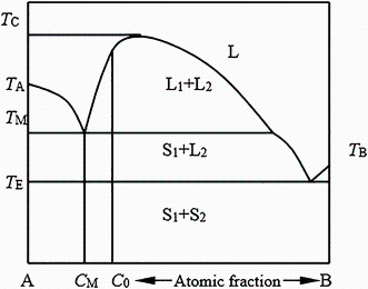
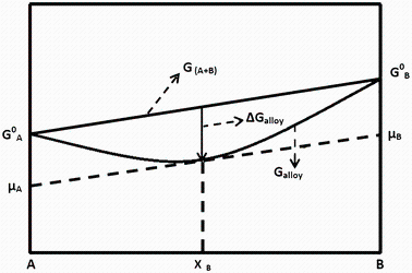
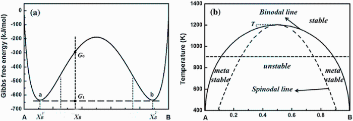
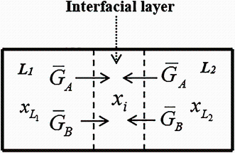
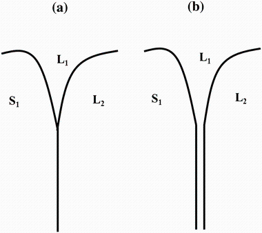
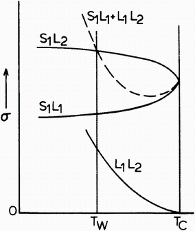
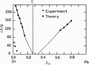
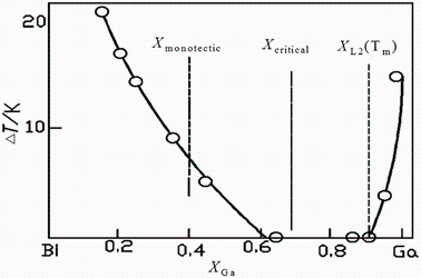
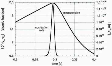
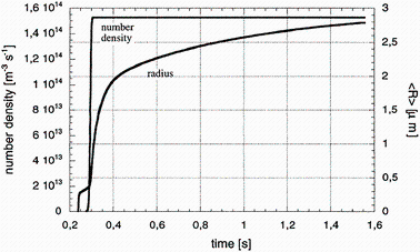
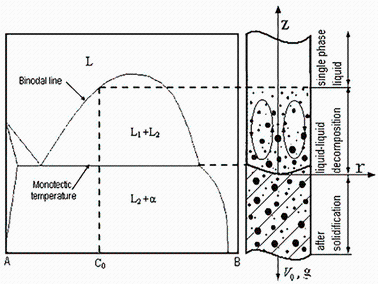
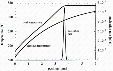
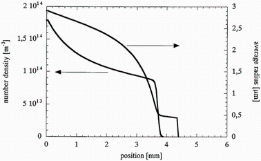
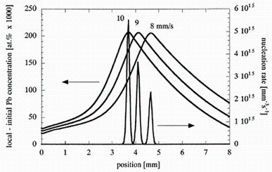
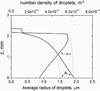
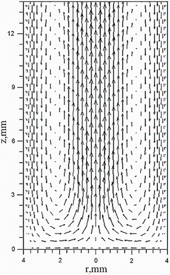
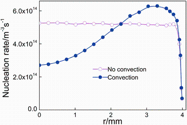
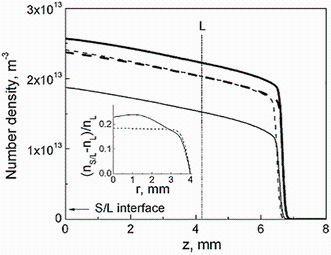
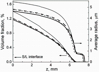
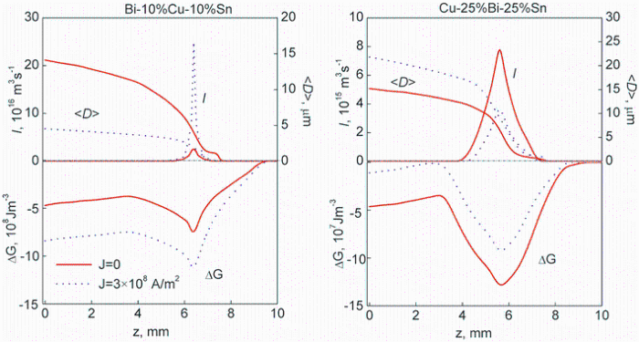
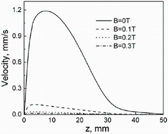
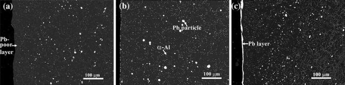
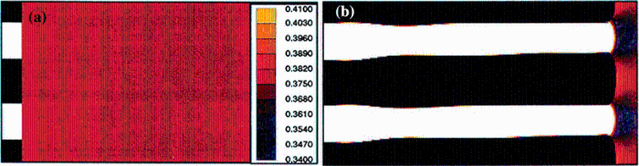
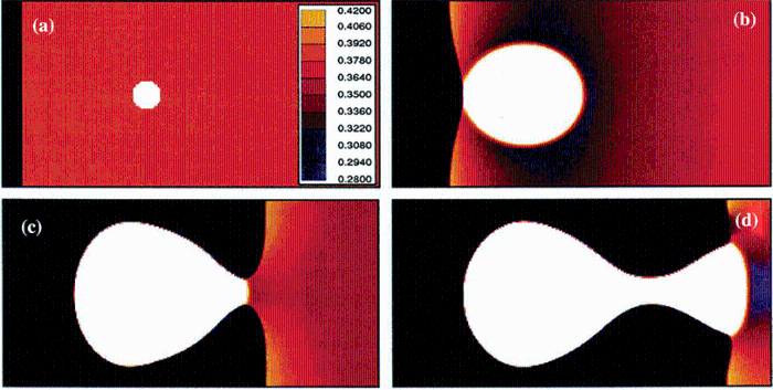
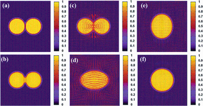
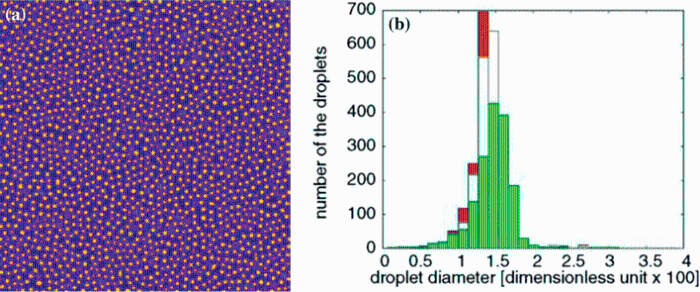
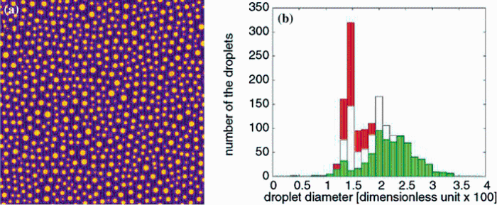
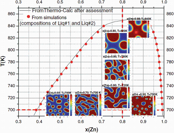

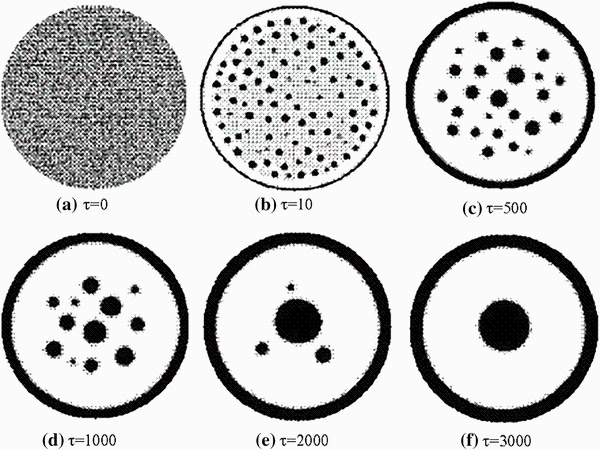