


An Algorithm to Analyze Electron Backscatter Diffraction Data for Grain Reconstruction: from Methodology to Application
[Xue-Hao Zheng1 , Hong-Wang Zhang1, 2  ]
]
]
|
|


An algorithm for grain reconstruction based on electron backscatter diffraction data was proposed in this paper. This algorithm can well record the original data arrangement when an external file for the reconstructed grain(s) was exported for further post-processing. Assisted by an in-house MATLAB program, grain reconstruction, lattice rotations, orientation spreads, and slip system analysis can be performed. The validity of this algorithm has been successfully tested by polycrystalline Ni before and after channel die compression.
Plastic deformation has been well recognized being heterogeneous, and different grains or different regions in individual grain usually undergo different deformations. As an example, Quey et al. [1] studied the average lattice rotations of each grain by using a split sample deformed by a series of compression in a channel die. They found that two grains of the same initial orientation but with different neighbors would rotate by angles that vary by 25% and axes separated by 37° on average. Thorning et al. [2] also revealed that a same grain was subdivided into domains with different lattice rotations owing to the grain interactions that are deviated from classical plasticity model predictions. Our recent investigations further demonstrated that the lattice rotations in a same grain are heterogeneous and the full-constraints Taylor model fails to predict the rotations of individual grains [3]. Therefore, studying the response of individual grains with different orientations to externally imposed strain and then evaluating the validity of the plasticity models calculation are of great scientific importance. Grain reconstruction in terms of individual orientations has become one of the primary but important steps to perform crystallographic analyses of plastic deformation at grain level.
Electron backscatter diffraction (EBSD) equipped in the scanning electron microscope (SEM) has become a powerful technique to characterize microstructural evolution [4], analyze lattice rotation [5], and predict the active slip systems[6]for crystalline materials. Many structural and textural parameters, such as grain size, grain area, boundary misorientation angle, volume fraction, and distribution of texture, can be conveniently obtained by commercial automatic data analysis software such as Oxford HKL and EDAX TSL. However, during grain reconstruction only the data corresponding to the reconstructed grain were saved, whereas the rest were totally omitted. As a result, when a new project for the reconstructed grain was generated, the regular grid mode (rectangle grid for HKL, rectangle and hexagonal grids for TSL) was lost, which does not allow orientation mapping being performed. Some open-source software packages offer grain reconstruction based on EBSD data, such as MTEX[7, 8] and VMAP [9, 10], but generation of a text-based file which can well record the original gird information for further analysis is not available. Some algorithms based on image processing [11, 12, 13, 14], however, does not allow orientation information being obtained. Consequently, an algorithm needs to be developed so as to overcome these shortcomings and to accurately address the grain rotation and/or orientation splitting during plastic deformation.
The present investigation will propose an algorithm for grain reconstruction based on EBSD data. The detailed position and orientation information in the scanned grid were accurately recorded when data were exported to an external text file, which permits the mapping operation as well as users’ customized controls. The algorithm, assisted by an in-house MATLAB program, has turned out to be successful to reconstruct grains, map the deformation-induced lattice rotations and orientation spreads for a polycrystalline Ni subjected to channel die compression.
The algorithm for grain reconstruction was developed to analyze the 2D data collected by EBSD scanned in a rectangular grid. An in-house MATLAB program called Grain_Reconstruction (The program packages are open-source and are available from the corresponding author on request.) implementing this algorithm has been developed to work with the EBSD data generated by the HKL Channel acquisition system and therefore only HKL Channel 5 software is used to compare with our in-house program in the following sections. The grain identification is performed based on the seed-filling algorithm [11, 15, 16] used widely in many areas of data and image analysis. The most significant difference between the present algorithm and the grain reconstruction used in the standard software is the way in which the data are stored. After grain reconstruction, data of the selected grain(s) can be saved and exported to a text-based file in which the data are arranged in the original grid. An example is shown in Table 1, where the data are corresponding to the Grain 1 in Fig. 1a. It is noted that the data of Grain 1 marked with a symbol “ √ ” as well as the remaining data marked with a symbol “ × ” but denoted as unresolved points are all saved, Fig. 1b. These unresolved points are characterized as a null phase represented by “ 0” in the second column of Table 1, and the corresponding Euler angle sets are all reset to zero. This is, however, quite different from that generated by HKL Channel 5 software, where only those data of Grain 1 are recorded and the remaining pixels marked with symbol “ × ” are totally omitted (Table 2).
| Table 1 Data for grain 1 in Fig. 1a exported by our in-house program |
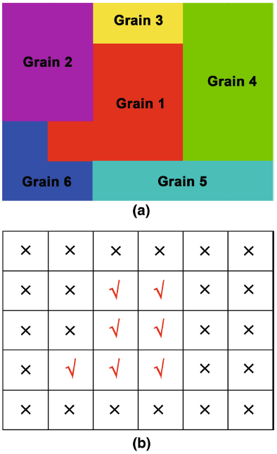 | Fig. 1 Schematic illustration of the grain reconstruction performed by Oxford HKL a and the corresponding scanned grid where six grains are indicated b. The pixels of grain 1 are highlighted and marked as a symbol “ √ ” and the remaining pixels are marked as a symbol “ × ” |
| Table 2 Data for grain 1 in Fig. 1a exported by HKL |
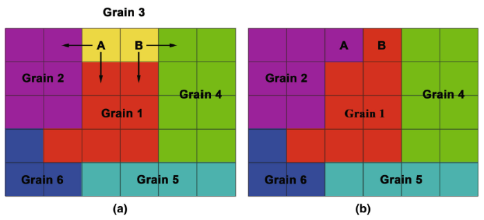
The misorientation angle is the key parameter for grain identification in the present method. A lower cutoff angle θ crit was preset (5° in the present investigation) to determine whether two adjacent pixels belong to the same grain or not. Besides, a grain must have an area larger than a critical area S crit (20 µ m2 in the present investigation), otherwise a grain reassignment is needed. There are two general cases for such a process: (1) a small grain is embedded in one large grain, and (2) it is surrounded by several large grains. For the first case, the small grain will be automatically assigned to the surrounding large one. For the second case, grain reassignment will be performed iteratively as follows. A 2D grain in the EBSD map can be geometrically viewed as stacking layers with one pixel in width and several pixels in length. If one pixel in the current layer has more neighboring pixels located in one neighboring large grain, this pixel would be assigned to this grain, otherwise this pixel is randomly assigned to the neighboring large grains. This process is continued until all the small grains are completely reassigned. An example is shown in Fig. 2a: Grain 3 (indicated by yellow color) is considered to be a small grain, and it is surrounded by three large grains: Grain 1, Grain 2 and Grain 4. Grain 3 consists of two pixels (marked by A and B, see Fig. 2a), and hence only one stacking layer with one pixel in width and two pixels in length needs to be considered. Specifically, pixel A has two neighboring pixels located, respectively, in Grain 1 and Grain 2; pixel B also has two neighboring pixels located in Grain 1 and Grain 4, respectively (see Fig. 2a). Due to their equal possibilities relative to their neighboring grains, pixels A and B are therefore randomly assigned to their neighboring large grains. One example is shown in Fig. 2b, where pixel A is assigned to Grain 2 and pixel B is assigned to Grain 1.
 | Fig. 2 Schematic illustrations of the grain maps before a after b the grain reassignment |
Our in-house MATLAB program provides several schemes to visualize reconstructed grains. One such approach is to plot the 3 Euler angles of each reconstructed grain using an RGB (red, green, blue) color scheme. The three Euler angles of each reconstructed grain can be obtained by calculating their average orientations via a quaternion method [17]. Due to the complete information on position, orientation, and grain index for each pixel, it is also allowed to visualizing the in-grain lattice rotation by correlating the orientations of pixels before and after deformation. Besides, the orientation spread, i.e., the orientation variations within each deformed grain from its average orientation, is also available. Apart from the aforementioned mapping schemes, the conventional functions of orientation mapping in HKL Channel 5 software can be used to process the exported file, giving rise to many other orientation maps, such as an All Euler map, inverse pole figure (IPF) map, and grain boundary map.
Generally, an individual grain does not deform as a unit but is subdivided into different domains with distinct dislocation structures [18, 19], crystallographic orientations [20, 21], and in-grain misorientation axes [22, 23]. Therefore, grain subdivision or orientation splitting requires quantitative investigation, in particular, for different isolated domains within one grain. The present algorithm provides an easy access to pick up these data of interest grain(s) so as to perform further post-analysis. Besides, other customized controls, such as constraints on grain size, grain shape, and Schmid factor, can be easily added into the algorithm.
A high-purity (99.96 wt%) polycrystalline nickel sample was chosen as the experimental material. The starting material was annealed at 850 ° C for 4 h, leading to near-equiaxed grains of about 100 μ m in size with weak crystallographic textures. The split-sample technique used in this study has been demonstrated to be able to follow grains in a polycrystal during large deformation[1, 24]. As illustrated in Fig. 3, a split sample with dimensions of 6 mm × 7 mm × 5 mm [rolling direction (RD) × transverse direction (TD) × normal direction (ND)] was used. It was made of two identical parts assembled along TD. The sample surfaces were mechanically polished, and both “ internal surfaces” were mechanically then electrolytically polished. An observation zone with an area of ~1 mm × 1 mm was marked by microhardness indentations on one of the internal surfaces. EBSD scanning with a step size of 5 μ m was first performed on the observation zone. Afterward, the two parts of the sample were glued together and subjected to channel die compression at a strain rate of 10-3 s-1 to a true strain of 0.20. The sample was lubricated using Teflon films and lubricating oil to minimize frictional effects during the deformation. The EBSD analysis of the deformed samples was carried out with a step size of 2 μ m on the same region.
 | Fig. 3 Schematic illustrations of the channel die compression and split-sample technique. The sample coordinate system is indicated |
Because of the limited angular resolution in EBSD [9], misorientation angles below a lower cutoff angle Δ θ , which depends on the EBSD systems and operating conditions, were disregarded. The selected Δ θ would influence the reconstructed microstructures and must be firstly considered. EBSD data collected from the initial sample were used to evaluate Δ θ . As shown in Fig. 4, the distribution of misorientation angles is independent of Δ θ when Δ θ ≥ 1.5° ; otherwise, a considerable amount of misorientation angles less than 3° are produced owing to the limited angular resolution of EBSD. Consequently, Δ θ was set to be 1.5° in the present investigation.
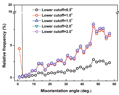 | Fig. 4 Influence of the distribution of misorientation angles by the lower cutoff angle |
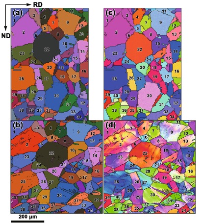
The above algorithm, assisted by our in-house MATLAB program, permits the grain reconstruction of the same region before (Fig. 5a) and after (Fig. 5b) deformation. The grain morphologies together with the deformation-induced geometrical change of given grains are well manifested. The reconstructed grain maps in Fig. 5a, b show a great similarity to the orientation maps obtained by HKL channel 5 software, Fig. 5c, d, and the grain size as well as the in-grain misorientations for the same grains is also highly consistent. It is therefore demonstrated that the present algorithm can provide identical grain information on grain area and in-grain misorientation as the HKL Channel 5 software.
 | Fig. 5 Reconstructed grain map of the sample before a, c and after deformation b, d by the present algorithm a, b and HKL Channel 5 software c, d, respectively. The black lines represent boundaries with misorientation angles larger than 5° . Grains in a, b are colored according to their average orientations (Euler contrast) while pixels in c, d are colored according to ND |
As shown in Fig. 5d, the color variation differs from grain to grain, implying a difference in the orientation change. The variations of orientation change have been attributed to the crystallographic orientation [25] as well as grain interaction[1, 2, 26, 27]. In this section, followed by the grain reconstruction, the in-grain lattice rotations will be extracted.
The in-grain lattice rotations in the deformed grains are expressed as axis/angle pairs (r, θ ) for each point with respect to the average orientations of the corresponding initial grains. Reconstructed grain maps were first performed, which are denoted as “ initial” and “ deformed” grain maps, respectively. The correlation between the “ initial” and the “ deformed” grain was built by arbitrarily clicking the same reconstructed grain on the “ initial” and the “ deformed” grain maps, respectively. Detailed procedures can refer to the user’ s manual attached to this in-house MATLAB program. Then the average orientation of the selected “ initial” grain together with the (r, θ ) pairs of each pixel will be calculated. The above process is repeated until all the interested grains are processed.
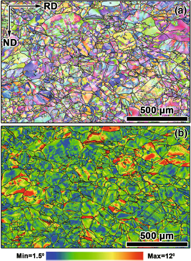
Rotation axes (r) were referred to the crystal coordinate system and were visualized by rotation axis maps (Fig. 6a) and stereographic projections (Fig. 6d). Instead of a RGB color scheme which cannot distinguish a rotation about +[uvw] from that about -[uvw][28, 29], a HSV (hue, saturation, value) color scheme was used to plot the rotation axis map for the 136 grains. Other similar color schemes can be found in the literature[29, 30, 31]; however, they are often a better choice for mapping rotation angle/axis or even five-parameter space of grain boundaries that includes the plane normal vectors. It should be noted that the rotation about [100] are less well visualized when the projection plane is 010-001, and this problem can be overcome by simultaneously providing rotation axis map color coded by the other projection planes (100-010 and 001-100).
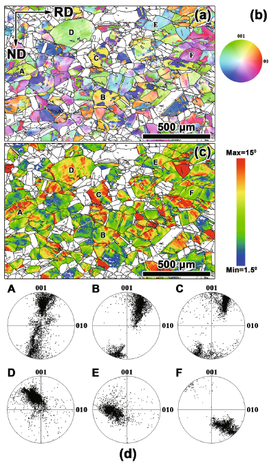
 | Fig. 6 Rotation axis map a and rotation angle map c for the 136 reconstructed grains. The color scheme used in a is shown in b. Stereographic projections of rotation axes for six typical grains (marked by “ A” -“ D” ) are shown in d. The black lines in a and c represent boundaries with misorientation angles larger than 5° |
As evidenced by Fig. 6a, an inhomogeneous distribution of rotation axes was revealed intuitively and vividly by the color variations in different grains. For example, grains “ A, ” “ B, ” and “ C” show a significant color variation, whereas grains “ D, ” “ E, ” and “ F” give rise to a roughly uniform color. The differences could be further evidenced by the stereographic projections shown by Fig. 6d which were reconstructed by the external files. The rainbow map (Fig. 6c) shows the distribution of rotation angles, a white color corresponding to a rotation angle ≤ 1.5° or non-reconstructed grains and a red color to rotation angles ≥ 15° . According to the color variation, the map also underpins the inhomogeneous distribution of the rotation angles in different grains or different parts of one grain. A comparison of the axis map and angle map, Fig. 6a, c, shows that the inhomogeneous distribution of rotation angles always comes with distinct variations of rotation axes. These observations are in qualitative accord with those reported in tensile-deformed polycrystalline copper [2], in which only one grain was followed at several successive strains.
It is therefore very convenient to obtain in-grain lattice rotations of a large amount of grains by the present algorithm. More specifically, the inhomogeneous lattice rotation was underpinned, which reflects the difference in the activated slip systems. Assisted by the quantitative information given by the present algorithm, the slip system analysis can be performed and will be exemplified by two typical grains “ B” and “ F.”
In fcc metals such as nickel, each of the 12 slip systems operating on {111} slip planes and along < 110> slip directions produces a crystal rotation about < 112> , i.e., a Taylor axis[32] which can be expressed as:
$$T = b^{\text{s}} \times n^{\text{s}}.(1)$$
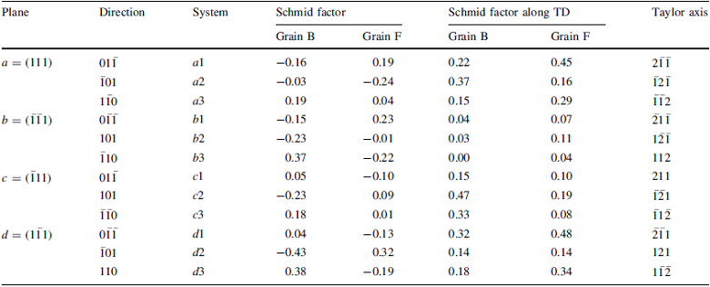
where bs and ns are the slip direction and slip plane normal, respectively, for a given slip system, s. The Taylor axes as well as the Schmid factors of the 12 slip systems in grain “ B” and grain “ F” are given in Table 3.
| Table 3 Schmid factors and Taylor axes of the 12 slip systems in grains “ B” and “ F” |
Due to the reaction stresses [33] imposed by the channel die, the potential active slip systems are b1, b2, b3, d2, and d3 in grain B and a2, b1, b3, and d2 in grain F. The practically active slip systems can be estimated based on the crystal rotation relative to the initial orientation by matching the Taylor axis for a given combination of slip systems to the experimentally measured lattice rotation axis[22, 34, 35].
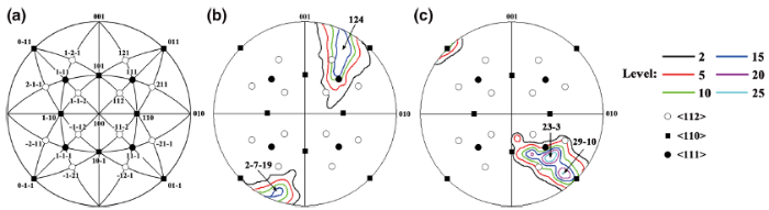
Figure 7a gives the positions of the < 112> , < 110> , and < 111> axes in the crystal coordinate system, where the traces of {111} slip planes and {110} planes are drawn as big black circles. For grain “ B” (Fig. 7b), lattice rotation axes display two peaks with identical intensities in the vicinities of [124] and \([2\bar{7}\bar{19}]\). This wide spectrum of lattice rotation axes corresponds well with its rotation axis map (Fig. 6a), in which the grain boundary regions show blue color whereas the grain interiors are colored by yellowish-brown. Analogously to the calculations in the Taylor/Bishop-Hill models[36], several combinations of slip systems with a geometrical lattice rotation axis deviating from the measured lattice rotation axis within a small angle can be obtained. In this study, a combination of slip systems minimizing the internal work is adopted, i.e., the slip systems which minimize total shear strains. As a result, a rotation axis around [124] resulted from the slip systems b2, b3, and d2 with a ratio of 1:6:1, while originated from b2, d2, and d3 with a ratio of 4:3:10.
 | Fig. 7 a Stereographic projection showing the < 110> , < 111> and < 112> directions in the crystal coordinate system. Contour maps with Miller indices corresponding to the maximum intensities highlight the distributions of rotation axes for grain “ B” b and grain “ F” c |
In the case of grain “ F” (Fig. 7c), the maximum intensities of lattice rotation axes are in the vicinities of \([23\bar{3}]\) and \([29\bar{10}]\). The maximum intensity of the lattice rotation axes for grain “ F” is higher than that of grain “ B, ” and its rotation axis map is also relatively uniform (Fig. 6a). A similar calculation shows that the unbalanced operation of slip systems a2, b3, and d2 has taken place for grain “ F.” Specifically, the rotation about \([23\bar{3}]\) and \([29\bar{10}]\) is induced by a2, b3, and d2 with a ratio of 3:9:10 and 1:10:10.
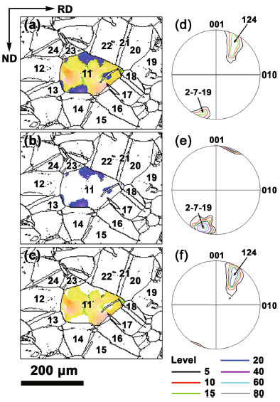
The above analysis indicates that different slip patterns are activated for grains “ B” and “ F.” For grain “ F, ” identical slip systems are activated in the whole grain, whereas for grain “ B, ” the activated slip systems varied from the grain interior to grain boundary areas. Through the data separation for grain “ B, ” Fig. 8, the lattice rotation axes around \([2\bar{7}\bar{1}\bar{9}]\) appear in the vicinities of the grain boundaries (Fig. 8b, e), whereas the rest of the grain mainly gives rise to the lattice rotation axes around [124] (Fig. 8c, f). This points to the influence of grain boundaries or adjacent grains on the activated slip systems, which agrees with the results in uniaxial deformed aluminum [34, 37].
 | Fig. 8 Rotation axis maps and the corresponding intensity contour maps of the whole grain a, d, grain boundary region b, e, and the rest of grain “ B” c, f, respectively |
The in-grain orientation spreads are quantified by calculating the misorientations of each point in deformed grains with respect to their average orientations, which can also be visualized by misorientation axis maps (Fig. 9a) and misorientation angle maps (Fig. 9b). The misorientation axes in some grains are relatively uniform, but in others are distributed in an inhomogeneous manner, forming several distinct regions (Fig. 9a). A similar pattern of heterogeneous fragmentation is also observed in misorientation angle maps (Fig. 9b). The grains exhibiting large variations of misorientation angles usually show large variations of misorientation axes (Fig. 9a). The visualization underpins the fact that a significant orientation spread has taken place even though the strain is pretty low. This non-uniform orientation spread in terms of misorientation axes and misorientation angles agrees with a report on polycrystalline Al-0.1%Mn during channel die compression [1].
 | Fig. 9 Misorientation axis map a and misorientation angle map b for grains with areas larger than 20 μ m2. Each color in a represents a specific misorientation axis between a pixel and the average orientation of the selected grain where the pixel is located. The color scheme used in a can be found in Fig. 6b. The black lines in a and b represent boundaries with misorientation angles larger than 5° |
The advantage of this algorithm is that it can reconstruct one or several grains and export the corresponding data to an external file with good records of the original grid of data arrangement. This feature, which cannot be achieved by the commercial software, allows the exported file to be routinely processed by conventional mapping functions supplemented in the commercial EBSD data processing software. Besides, crystallographic analyses of plastic deformation at grain level in terms of grain identification, in-grain lattice rotations, orientation spreads and prediction of slip system can be performed by our in-house Matlab program implementing this algorithm. This algorithm at present can only process 2D orientation data collected from a single phase with a cubic crystal structure. One of our on-going projects is to explore the algorithm for other metals with different crystal structures and phase constitutions as well as the analysis of orientation data arranged in 3D.
An algorithm for grain reconstruction based on EBSD data has been developed. Compared with grain reconstruction by commercial EBSD software, this algorithm can record the original grid of data arrangement. This allows post-data-processing such as in-grain lattice rotations and orientation spreads together with a slip system analysis being readily performed assisted by an in-house MATLAB program. The validity of this algorithm has been successfully testified by a polycrystalline Ni sample before and after channel die compression.
Footnotes1The program packages are open-source and are available from the corresponding author on request.
The authors thank Prof. Brian Ralph for useful comments on the manuscript. The authors also gratefully acknowledge the financial support of the Ministry of Science and Technology of China (Grant No. 2012CB932201), the National Natural Science Foundation of China (Grant Nos. 51231006 and 51171182), and the Danish-Chinese Center for Nanometals (Grant Nos. 51261130091 and DNRF86-5).
The authors have declared that no competing interests exist.
| [1] |
|
| [2] |
|
| [3] |
|
| [4] |
|
| [5] |
|
| [6] |
|
| [7] |
|
| [8] |
|
| [9] |
|
| [10] |
|
| [11] |
|
| [12] |
|
| [13] |
|
| [14] |
|
| [15] |
|
| [16] |
|
| [17] |
|
| [18] |
|
| [19] |
|
| [20] |
|
| [21] |
|
| [22] |
|
| [23] |
|
| [24] |
|
| [25] |
|
| [26] |
|
| [27] |
|
| [28] |
|
| [29] |
|
| [30] |
|
| [31] |
|
| [32] |
|
| [33] |
|
| [34] |
|
| [35] |
|
| [36] |
|
| [37] |
|